Chapter 6, Animint options
This chapter gives a complete list of new features that animint introduces to the grammar of graphics. After reading this chapter, you will understand how to customize your animint graphics via
- the
href,tooltip,idaesthetics for observation-specific characteristics; - named elements of
clickSelectsandshowSelectedfor specifying several selection variables at once; - the
chunk_varsgeom-specific option; - the
color_off,fill_off, andalpha_offgeom parameters for specifying how selection state is displayed; - the
helpandtitlegeom-specific parameters, which can be set to text strings that will be shown in the guided tour. - plot-specific legends and height/width options; and
- global data viz options.
Observation-specific options (new aesthetics)
This section explains the new aesthetics that are recognized by animint2.
Review of previously introduced aesthetics
First we discuss the new aesthetics that we have already introduced in previous chapters.
Chapter 3 also introduced aes(key) to designate a variable to use for smooth transitions that are interpretable.
Hyperlinks using aes(href)
The code below uses animint to draw a map of the United States.
library(animint2)
USpolygons <- map_data("state")
animint(
  map=ggplot()+
    ggtitle("click a state to read its Wikipedia page")+
    coord_equal()+
    geom_polygon(aes(
      x=long, y=lat, group=group,
      href=paste0("http://en.wikipedia.org/wiki/", region)),
      data=USpolygons, fill="black", colour="grey"))
Try clicking a state in the data viz above. You should see the corresponding wikipedia page open in a new tab.
Tooltips using aes(tooltip)
Tooltips are little windows of text information that appear when you hover the cursor over something on the screen. In animint you can use aes(tooltip) to designate the observation-specific message that appears. For example we use it to display the population and country name in the scatterplot of the World Bank data below.
data(WorldBank)
WorldBank1975 <- subset(WorldBank, year == 1975)
animint(
  scatter=ggplot()+
    geom_point(aes(
      x=life.expectancy, y=fertility.rate,
      tooltip=paste(country, "population =", population)),
      size=5,
      data=WorldBank1975))
Try hovering the cursor over one of the data points. You should see a small box appear with the country name and population for that data point.
Note that a tooltip of the form “variable value” is specified by default for each geom with aes(clickSelects). For example a geom with aes(clickSelects=year) shows the default tooltip “year 1984” for an observation with year 1984. You can change this default by explicitly specifying aes(tooltip).
HTML id attribute using aes(id)
Since everything plotted by animint is rendered as an SVG element in a web page, you may want to specify a HTML id attribute using aes(id) as below.
animint(
  map=ggplot()+
    ggtitle("each state/region/group has a unique id")+
    coord_equal()+
    geom_polygon(aes(
      x=long, y=lat, group=group,
      id=gsub(" ", "_", paste(region, group))),
      data=USpolygons, fill="black", colour="grey"))
Note how gsub is used to convert spaces to underscores, since a well-defined id must not include spaces. Note also that paste is used to add a group number, since there may be more than one polygon per state/region, and each id must be unique on a web page. The animint2 developers use this feature for testing the animint JavaScript renderer code.
Data-driven selector names using named clickSelects and showSelected
Chapter 3 introduced showSelected for designating a geom which shows only the selected subset of its data.
Chapter 4 introduced clickSelects to designate a geom which can be clicked to change a selection variable.
Usually selector names are defined in showSelected or clickSelects. For example, showSelected=c("year", "country") means to create two selection variables (named year and country). However, that method becomes inconvenient if you have many selectors in your data viz. To illustrate we consider the following theoretical example (the code in this section is not directly executable). Say you want to use 20 different selector variable names, selector1value … selector20value. The usual way to define your data viz would be
viz <- list(
  points=ggplot()+
    geom_point(clickSelects="selector1value", data=data1)+
    ...
    geom_point(clickSelects="selector20value", data=data20)
)
However that method is bad since it violates the DRY principle (Don’t Repeat Yourself). Another way to do that would be to use a for loop:
viz <- list(points=ggplot())
for(selector.name in paste0("selector", 1:20, "value")){
  data.for.selector <- all.data.list[[selector.name]]
  viz$points <- viz$points +
    geom_point(clickSelects=selector.name, data=data.for.selector)
}
That method is bad since it is slow to construct viz, and the compiled viz potentially takes up a lot of disk space since there is at least one TSV file created for each geom_point. The preferable method is to use a named character vector for clickSelects. The names should be used to indicate the column that contains the selector variable name. For example:
viz <- list(
  points=ggplot()+
    geom_point(
      clickSelects=c(selector.name="selector.value"),
      data=all.data)
)
The animint compiler looks through the data.frame all.data and create selectors for each of the distinct values of all.data$selector.name. Clicking one of the data points updates the corresponding selector with the value indicated in all.data$selector.value.
You can similarly use one geom with a named showSelected instead of a bunch of different geoms with showSelected.
This feature is useful not only to avoid repetition in the definition of the data viz, but also because they are more computationally efficient. For a detailed example with timings and disk space measurements, see Chapter 14.
Geom options
In animint, there are several options for customization at the geom level: chunk_vars is used to specify how to split data sets for storage on disk, and *_off parameters are used to specify how a clickSelects geom should be displayed when it is not selected. Additionally, help and title may be specified, to add information to the guided tour.
The chunk_vars geom-specific compilation option
The chunk_vars option defines the selection variables that are used to split the data set into separate chunks (TSV files) to download. There is one TSV file created for each combination of values of the chunk_vars variables. More selection variables specified in chunk_vars means to split the data set into more TSV files, each of a smaller size.
The chunk_vars option should be specified as an argument to a geom_* function, and its value should be a character vector of selection variable names. When chunk_vars=character(0), a character vector of length zero, all of the data is stored in a single TSV file. When chunk_vars is set to all of the showSelected variable names, then a TSV file is created for each combination of values of those variables.
In general the animint compiler chooses a sensible default for chunk_vars, but you may want to specify chunk_vars if the data viz is loading slowly, or taking up too much space on disk. If the data viz is loading slowly, you should add selection variables to chunk_vars to reduce the size of the first TSV file to download. If the data viz takes up too much space on disk, you should remove selection variables from chunk_vars to decrease the number of TSV files. Lots of small TSV files can take more disk space than a single TSV file because some filesystems store a constant amount of metadata for every file.
To illustrate the usage of chunk_vars, consider the following visualization of the breakpoints data set.
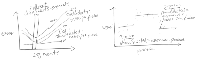
The sketch above consists of two plots. We begin by creating the plot of error curves on the left.
data(breakpoints)
only.error <- subset(breakpoints$error, type=="E")
only.segments <- subset(only.error,bases.per.probe==bases.per.probe[1])
library(data.table)
fp.fn.names <- rbind(
  data.table(error.type="false positives", type="FP"),
  data.table(error.type="false negatives", type=c("I", "FN")))
error.dt <- data.table(breakpoints$error)
error.type.dt <- error.dt[fp.fn.names, on=list(type)]
fp.fn.dt <- error.type.dt[, list(
  error.value=sum(error)
), by=.(error.type, segments, bases.per.probe)]
errorPlot <- ggplot()+
  ggtitle("select data and segments")+
  theme_bw()+
  geom_tallrect(aes(
    xmin=segments-0.5, xmax=segments+0.5),
    clickSelects="segments",
    data=only.segments,
    alpha=1/2)+
  geom_line(aes(
    segments, error.value, color=error.type,
    group=paste(bases.per.probe, error.type)),
    showSelected="bases.per.probe",
    data=fp.fn.dt,
    size=5)+
  scale_color_manual(values=c(
    "false positives"="red", "false negatives"="blue"))+
  geom_line(aes(
    segments, error, group=bases.per.probe),
    clickSelects="bases.per.probe",
    data=only.error,
    size=4)+
  scale_x_continuous(breaks=c(1, 6, 10, 20))
errorPlot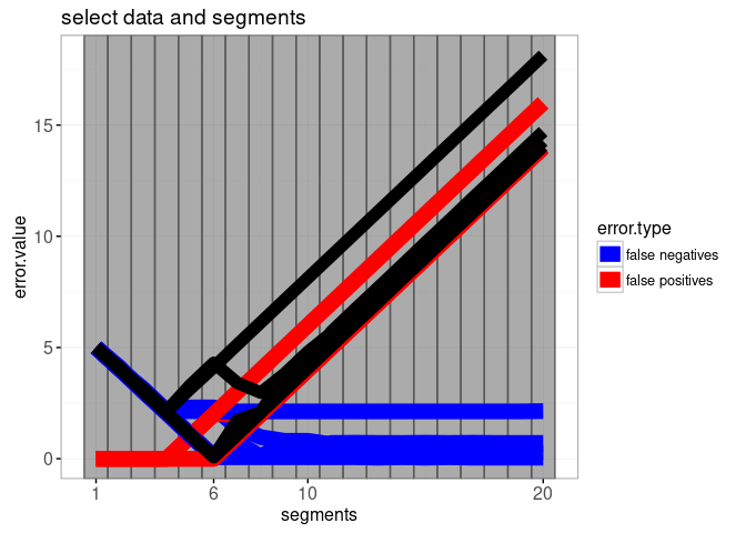
The plot above includes a geom_tallrect with clickSelects=segments and a geom_line with clickSelects=bases.per.probe. It will be used to select the data and model in the plot below.
signalPlot <- ggplot()+
  theme_bw()+
  theme(panel.margin=grid::unit(0, "lines"))+
  theme_animint(height=800)+
  geom_point(aes(
    position/1e5, signal),
    showSelected="bases.per.probe",
    shape=1,
    data=breakpoints$signals)+
  geom_segment(aes(
    first.base/1e5, mean, xend=last.base/1e5, yend=mean),
    showSelected=c("segments", "bases.per.probe"),
    color="green",
    data=breakpoints$segments)
signalPlot+facet_grid(segments ~ bases.per.probe)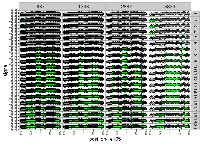
The non-interactive plot above has 80 facets, one for each combination of the two showSelected variables, bases.per.probe and segments. Below we make an interactive version in which only one of these facets will be shown.
(viz.chunk.vars <- animint(
  errorPlot,
  signal=signalPlot+
    geom_vline(aes(
      xintercept=base/1e5),
      showSelected=c("segments", "bases.per.probe"),
      color="green",
      chunk_vars=character(),
      linetype="dashed",
      data=breakpoints$breaks)))
Click the “Show download status table” button, and you should see counts of chunks (TSV files). Note that geom6_vline_signal has only 1 chunk, since chunk_vars=character() is specified for the geom_vline in the R code above. If another value of chunk_vars was specified, it would create a different number of TSV files, but the appearance of the data viz should be the same.
Below we use the du command line program to determine the disk usage of the data viz for different choices of chunk_vars.
tsvSizes <- function(segment.chunk.vars){
  viz <- list(
    error=errorPlot,
    signal=signalPlot+
      geom_vline(aes(
        xintercept=base/1e5),
        showSelected=c("segments", "bases.per.probe"),
        color="green",
        chunk_vars=segment.chunk.vars,
        linetype="dashed",
        data=breakpoints$breaks)
  )
  info <- animint2dir(viz, open.browser=FALSE)
  cmd <- paste("du -ks", info$out.dir)
  kb.dt <- fread(cmd=cmd)
  setnames(kb.dt, c("kb", "dir"))
  tsv.vec <- Sys.glob(paste0(info$out.dir, "/*.tsv"))
  is.geom6 <- grepl("geom6", tsv.vec)
  data.frame(kb=kb.dt$kb, geom6.tsv=sum(is.geom6), other.tsv=sum(!is.geom6))
}
chunk_vars_list <- list(
  neither=c(),
  bases.per.probe=c("bases.per.probe"),
  segments=c("segments"),
  both=c("segments", "bases.per.probe"))
sizes.list <- lapply(chunk_vars_list, tsvSizes)
(sizes <- do.call(rbind, sizes.list))
## kb geom6.tsv other.tsv
## neither 712 1 12
## bases.per.probe 716 5 12
## segments 772 19 12
## both 1000 76 12The table above includes counts of kilobytes for the data viz, along with counts of TSV files for geom6_vline_signal and the other geoms. Note how the choice of chunk_vars affects the number of TSV files and the disk space usage. Since chunk_vars was only specified for geom6_vline_signal, the number of TSV files for the other geoms does not change. When both segments and bases.per.probe are specified for chunk_vars, there are 76 TSV files for geom6_vline_signal, and the data viz takes 1000 kilobytes. In contrast, chunk_vars=character() produces only one TSV file for geom6_vline_signal, and the data viz uses 712 kilobytes.
In conclusion, the geom-specific chunk_vars option defines the number of TSV files created for each geom. When deciding the value of chunk_vars, you should consider both disk usage and loading time. A few large files take up less disk space but are slower to download than many small files.
Specifying how selection state is displayed
Animint has sensible defaults for displaying selection state. In particular,
- when there is a rect or tile with clickSelects, we use black color/border to show items which are selected, and transparent for items which are not selected.
- for any other geom with clickSelects, we use full opacity
alphato show items which are selected, andalpha-0.5opacity to show items which are not selected.
The defaults explained above are illustrated in the first plot below. Those defaults may be customized by using the alpha_off, fill_off, and color_off geom parameters as in the code below,
N <- 3
set.seed(1)
demo_df <- data.frame(i=1:N, num=rnorm(N,2))
animint(
  defaults=ggplot()+
    ggtitle("Defaults, no *_off")+
    geom_tile(aes(
      i, 0),
      size=5,
      clickSelects="i",
      data=demo_df)+
    geom_point(aes(
      i, num),
      size=5,
      clickSelects="i",
      data=demo_df),
  off=ggplot()+
    ggtitle("User specified alpha_off, fill_off, color_off")+
    geom_tile(aes(
      i, 0, fill=i),
      clickSelects="i",
      color="red",
      color_off="pink",
      size=5,
      data=demo_df)+
    geom_point(aes(
      i, num),
      size=5,
      alpha=0.5,
      alpha_off=0.1,
      clickSelects="i",
      data=demo_df)+
    geom_point(aes(
      i, -num),
      size=5,
      alpha=1,
      alpha_off=1,
      color="red",
      color_off="black",
      fill="grey",
      fill_off="white",
      clickSelects="i",
      data=demo_df))
Note that when using any one of these visual properties in the aes mapping, it should not be specified as a geom parameter. For example in the tile above, we used aes(fill), so fill and fill_off should not be specified as parameters for that geom (in order to make it clear that fill is used for displaying data values, not selection state).
Specifying guided tour text
Since Jan 2025, animint supports a guided tour, which displays information about possible interactions with each geom. To customize what is displayed for each geom, you can specify the help and title parameters, as in the code below.
animint(
  scatter=ggplot()+
    geom_point(aes(
      x=life.expectancy, y=fertility.rate, color=region),
      size=5,
      showSelected="year",
      clickSelects="country",
      help="One point drawn for each country in the selected year",
      alpha=0.7,
      data=WorldBank)+
    geom_text(aes(
      x=life.expectancy, y=fertility.rate, label=country),
      data=WorldBank,
      title="Selected country",
      showSelected=c("year","country")),
  first=list(
    country="France",
    year=1980))
In the code above, we specify help for geom_point, which controls the sub-text which is displayed for that geom, after clicking the “Start Tour” button at the bottom of the data visualization. After clicking the “Next” button, we can see the title that was specified in the code, shown at the top of the tour window, for the geom_text. This mechanism can be used to provide extra helpful information for the users of your data visualization, so they can more easily understand what is displayed, and what interactions are possible.
Plot-specific options
This section discusses options which are specific to one ggplot of a data viz. The theme_animint function is used to attach animint options to ggplot objects.
Plot height and width
The width and height options are for specifying the dimensions (in pixels) of a ggplot rendered by animint. For example, consider the following re-design of the plot of the United States:
animint(
  map=ggplot()+
    theme_animint(width=750, height=500)+
    theme(
      axis.line=element_blank(),
      axis.text=element_blank(),
      axis.ticks=element_blank(),
      axis.title=element_blank(),
      panel.border=element_blank(),
      panel.background=element_blank(),
      panel.grid.major=element_blank(),
      panel.grid.minor=element_blank())+
    geom_polygon(aes(
      x=long, y=lat, group=group),
      data=USpolygons, fill="black", colour="grey"))
Note that the plot above was rendered with a width of 750 pixels and a height of 500 pixels, due to the theme_animint options. If either of these options is not specified for any ggplot, then animint uses a default of 400 pixels.
Also note that theme was used to specify several blank elements. This has the effect of removing the axes and background, and is generally useful for rendering maps.
Size scale in pixels
The scale_size_animint scale should be used in all ggplots where you specify aes(size). To see why, consider the following examples.
scatter1975 <- ggplot()+
  geom_point(
    aes(x=life.expectancy, y=fertility.rate, size=population),
    WorldBank1975,
    shape=21,
    color="red",
    fill="black")
(viz.scale.size <- animint(
  ggplotDefault=scatter1975+
    ggtitle("no scale specified"),
  animintDefault=scatter1975+
    ggtitle("scale_size_animint()")+
    scale_size_animint(),
  animintOptions=scatter1975+
    ggtitle("scale_size_animint(pixel.range, breaks)")+
    scale_size_animint(pixel.range=c(5, 15), breaks=10^(10:1))))
The first ggplot above has no scale specified, so it uses the default ggplot2 scale, which has two problems. The first problem is that it seems that all countries have about the same size except the two really big countries. That problem can be fixed by simply adding scale_size_animint() to the ggplot, which results in the second plot above. However, a second problem is that the legend entries do not show the full range of the data. That problem is fixed in the third plot above, by manually specifying the breaks to use for legend entries. Note that the pixel.range argument can also be used to specify the radius of the largest and smallest circles.
Axes and legend text size
The syntax of defining axes and legend text size(in pixels) is almost the same as ggplot2. Inside theme, you can use numbers directly to change the font size, or you can use rel() to define the relative size.
scatter1975 <- ggplot()+
  geom_point(aes(
    x=life.expectancy, y=fertility.rate, color=region),
    data=WorldBank1975)
(viz.text.size <- animint(
  animintDefault=scatter1975+
    theme_animint(width=500, height=500)+
    ggtitle("no axes and legend size specified"),
  animintAxesOptions=scatter1975+
    theme_animint(width=500, height=500)+
    theme(axis.text=element_text(size=20))+
    ggtitle("axis.text=element_text(size=20)"),
  animintLegendOptions=scatter1975+
    theme_animint(width=500, height=500)+
    theme(
      legend.title=element_text(size=24),
      legend.text=element_text(size=rel(2.5)))+
    ggtitle("legend.text=element_text(size=rel(2.5)")))
This allows you to change the font size while changing the size of the plot to make it look more coherent.
Note that the default font size in animint is 11px for the axes and 16px for the legend.
Global data viz options
Global data viz options are any named elements of the viz list that are not ggplots.
Review of previously introduced global options
Chapter 3 introduced the duration option for specifying the duration of smooth transitions.
Chapter 3 introduced the time option for specifying a selection variable which is automatically updated (animation).
Chapter 4 introduced the first option for specifying the selection when the data viz is first rendered.
Chapter 4 introduced the selector.types option for specifying multiple selection variables.
Web page title with the title option
The title option should be a character string, and will be used to set the <title> element of the web page. It does not make sense to use the title option in an Rmd document such as this page. A title can and should be used with animint2dir, as in the code below.
viz.title <- viz.scale.size
viz.title$title <- "Several size scales"
animint2dir(viz.title, "Ch06-title")
Note that viz.scale.size already has three ggplots, each with a ggtitle. Adding the global title option has the effect of defining a title for the web page.
Chapter 5 introduced the animint2pages function, which is used to publish an animint to GitHub Pages. It requires that the animint defines the title option, because that meta-data is required for organizing the animint in a gallery.
Link R code with source option
The source option should be a character string: a link to the R source code which was used to create the animint.
animint(
  demo=ggplot()+
    geom_point(aes(
      Petal.Length, Sepal.Length),
      data=iris),
  source="https://github.com/tdhock/animint-book/edit/master/Ch06-other.Rmd")
Note above how there is a source link at the bottom of the data viz.
Chapter 5 introduced the animint2pages function, which is used to publish an animint to GitHub Pages. It requires that the animint defines the source option, because that meta-data is required for organizing the animint in a gallery.
Link a video
The video option should be a character string: a link to a video which shows typical interactions with the animint. This mechanism can be used to help the users of your data visualization understand what is displayed, and what interactions they can use.
animint(
  video="https://vimeo.com/1050117030",
  scatter=ggplot()+
    geom_point(aes(
      x=life.expectancy, y=fertility.rate, color=region),
      clickSelects="country",
      alpha=0.7,
      data=WorldBank1975))
In the data visualization above, notice the “video” link which appears in the bottom right. Clicking that link leads to a video that was recorded to explain a more complex data visualization based on the World Bank data. The idea is that you can record a video for each of your animints, and then include a link to the video using this mechanism, so your users can more easily understand what is displayed, and what interactions are possible.
Show or hide selection menus with the selectize option
The selectize option should be a named list of logical values. Names should be selector variables, and values should indicate whether or not you would like to render a selection menu via selectize.js. By default, animint will render a selection menu for every selection variable, with two exceptions:
- data-driven selection variables that are defined using named clickSelects/showSelected variables.
- selection variables that have a lot of values (they are slow to render).
These defaults should work well for the vast majority of animints. For those who are interested to see an example of how the selectize option works, please see the PredictedPeaks test in the animint2 source code.
Chapter summary and exercises
This chapter explained several options for customizing animints at the observation, geom, plot, and global level.
Exercises:
- Create other versions of
viz.chunk.varswith different values ofchunk_varsfor thegeom_pointandgeom_segment. How does the choice ofchunk_varsaffect the appearance of the visualization? The disk space? The loading time?
Next, Chapter 7 explains the limitations of the current implementation of animint2.
