Chapter 18, Neural networks
In this chapter we will explore several data visualizations of the gradient descent learning algorithm for Neural networks.
Chapter outline:
- We begin by simulating and visualizing some 2d data for binary classification.
- We then show how a classification function in 2d can be visualized by computing predictions on a grid, and then using
geom_tileorgeom_pathwith contour lines. - We compute linear model predictions, and gradient descent updates, using a simple automatic differentiation (auto-grad) system.
- We end by implementing gradient descent for a neural network, and using an interactive data visualization to show how the predictions get more accurate with iterations of the learning algorithm.
Visualize simulated data
In this section, we simulate a simple data set with a non-linear pattern for binary classification.
sim.col <- 2
sim.row <- 100
set.seed(1)
features.hidden <- matrix(runif(sim.row*sim.col), sim.row, sim.col)
head(features.hidden)
## [,1] [,2]
## [1,] 0.2655087 0.6547239
## [2,] 0.3721239 0.3531973
## [3,] 0.5728534 0.2702601
## [4,] 0.9082078 0.9926841
## [5,] 0.2016819 0.6334933
## [6,] 0.8983897 0.2132081In the simulation, the data table above has the “hidden” features which are used to create the labels, but are not available for learning. The latent/true function used for classification is the following,
bayes <- function(DT)DT[, (V1>0.2 & V2<0.8)]
library(data.table)
hidden.dt <- data.table(features.hidden)
label.vec <- ifelse(bayes(hidden.dt), 1, -1)
table(label.vec)
## label.vec
## -1 1
## 31 69The binary labels above are created from the hidden features, but for learning we only have access to the noisy features below,
set.seed(1)
features.noisy <- features.hidden+rnorm(sim.row*sim.col, sd=0.05)
head(features.noisy)
## [,1] [,2]
## [1,] 0.2341860 0.6237056
## [2,] 0.3813061 0.3553031
## [3,] 0.5310719 0.2247141
## [4,] 0.9879718 1.0005855
## [5,] 0.2181573 0.6007640
## [6,] 0.8573663 0.3015725To plot the data and visualize the pattern, we use the code below,
library(animint2)
label.fac <- factor(label.vec)
sim.dt <- data.table(features.noisy, label.fac)
ggplot()+
  geom_point(aes(
    V1, V2, color=label.fac),
    data=sim.dt)+
  coord_equal()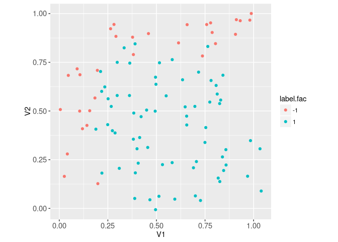
The plot above shows each row in the data set as a point, with the two features on the two axes, and the two labels in two different colors. The lower right part of the feature space tends to have positive labels, and the left and top areas have negative labels. This is the pattern that the neural network will learn. To properly train a neural network, we need to split the data into two sets:
- subtrain: used to compute gradients, which are used to update weight parameters, and predicted values. With enough iterations/epochs of the gradient descent learning algorithm, and a powerful enough neural network model (large enough number of hidden units/layers), it should be possible to get perfect prediction on the subtrain set.
- validation: used to avoid overfitting. By computing the prediction error on the validation set, and choosing the number of gradient descent iterations/epochs which minimizes the validation error, we can ensure the learned model has good generalization properties (provides good predictions on not only the subtrain set, but also new data points like in the validation set).
is.set.list <- list(
  validation=rep(c(TRUE,FALSE), l=nrow(features.noisy)))
is.set.list$subtrain <- !is.set.list$validation
set.vec <- ifelse(is.set.list$validation, "validation", "subtrain")
table(set.vec)
## set.vec
## subtrain validation
## 50 50The code above is used to randomly assign half of the data into each of the subtrain and validation sets. Below, we plot the two sets in separate facets,
sim.dt[, set := set.vec]
ggplot()+
  facet_grid(. ~ set, labeller=label_both)+
  geom_point(aes(
    V1, V2, color=label.fac),
    data=sim.dt)+
  coord_equal()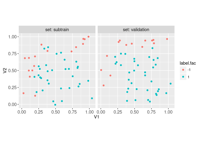
Visualize Bayes optimal classification function
To visualize the optimal/Bayes decision boundary, we need to evaluate the function on a 2d grid of points that spans the feature space. To create such a grid, we first create a list which contains the two 1d grids for each feature,
(grid.list <- lapply(sim.dt[, .(V1, V2)], function(V){
  seq(min(V), max(V), l=30)
}))
## $V1
## [1] 0.005600558 0.041238397 0.076876237 0.112514077 0.148151916 0.183789756
## [7] 0.219427595 0.255065435 0.290703274 0.326341114 0.361978954 0.397616793
## [13] 0.433254633 0.468892472 0.504530312 0.540168151 0.575805991 0.611443831
## [19] 0.647081670 0.682719510 0.718357349 0.753995189 0.789633028 0.825270868
## [25] 0.860908708 0.896546547 0.932184387 0.967822226 1.003460066 1.039097905
##
## $V2
## [1] -0.006562821 0.028166431 0.062895684 0.097624936 0.132354189
## [6] 0.167083441 0.201812694 0.236541946 0.271271199 0.306000451
## [11] 0.340729703 0.375458956 0.410188208 0.444917461 0.479646713
## [16] 0.514375966 0.549105218 0.583834471 0.618563723 0.653292975
## [21] 0.688022228 0.722751480 0.757480733 0.792209985 0.826939238
## [26] 0.861668490 0.896397742 0.931126995 0.965856247 1.000585500Then we use CJ (cross-join) to create a data table representing the 2d grid, for which we evaluate the best/Bayes classification function,
(grid.dt <- do.call(
  CJ, grid.list
)[
, bayes.num := ifelse(bayes(.SD), 1, -1)
][
, bayes.fac := factor(bayes.num)
][])
## Key: <V1, V2>
## V1 V2 bayes.num bayes.fac
## <num> <num> <num> <fctr>
## 1: 0.005600558 -0.006562821 -1 -1
## 2: 0.005600558 0.028166431 -1 -1
## 3: 0.005600558 0.062895684 -1 -1
## 4: 0.005600558 0.097624936 -1 -1
## 5: 0.005600558 0.132354189 -1 -1
## ---
## 896: 1.039097905 0.861668490 -1 -1
## 897: 1.039097905 0.896397742 -1 -1
## 898: 1.039097905 0.931126995 -1 -1
## 899: 1.039097905 0.965856247 -1 -1
## 900: 1.039097905 1.000585500 -1 -1The best classifier is visualized below in the feature space,
ggplot()+
  geom_tile(aes(
    V1, V2, fill=bayes.fac),
    color=NA,
    data=grid.dt)+
  geom_point(aes(
    V1, V2, fill=label.fac),
    color="black",
    shape=21,
    data=sim.dt)+
  coord_equal()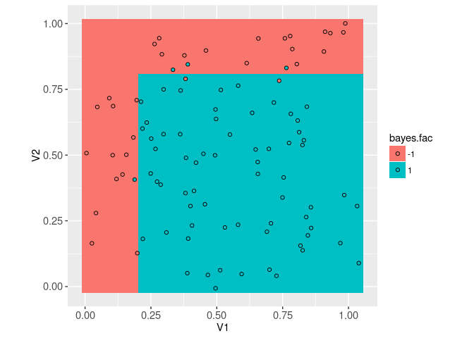
The plot above shows that even using the best possible function, there are still some prediction errors (points on a background of different color). Another way to visualize that best classification function is via the decision boundary, which can be computed using the code below,
get_boundary <- function(score){
  contour.list <- contourLines(
    grid.list$V1, grid.list$V2,
    matrix(score, length(grid.list$V1), length(grid.list$V2), byrow=TRUE),
    levels=0)
  if(length(contour.list)){
    data.table(contour.i=seq_along(contour.list))[, {
      with(contour.list[[contour.i]], data.table(level, x, y))
    }, by=contour.i]
  }
}
(bayes.contour.dt <- get_boundary(grid.dt$bayes.num))
## contour.i level x y
## <int> <num> <num> <num>
## 1: 1 0 0.2016087 -0.006562821
## 2: 1 0 0.2016087 0.028166431
## 3: 1 0 0.2016087 0.062895684
## 4: 1 0 0.2016087 0.097624936
## 5: 1 0 0.2016087 0.132354189
## 6: 1 0 0.2016087 0.167083441
## 7: 1 0 0.2016087 0.201812694
## 8: 1 0 0.2016087 0.236541946
## 9: 1 0 0.2016087 0.271271199
## 10: 1 0 0.2016087 0.306000451
## 11: 1 0 0.2016087 0.340729703
## 12: 1 0 0.2016087 0.375458956
## 13: 1 0 0.2016087 0.410188208
## 14: 1 0 0.2016087 0.444917461
## 15: 1 0 0.2016087 0.479646713
## 16: 1 0 0.2016087 0.514375966
## 17: 1 0 0.2016087 0.549105218
## 18: 1 0 0.2016087 0.583834471
## 19: 1 0 0.2016087 0.618563723
## 20: 1 0 0.2016087 0.653292975
## 21: 1 0 0.2016087 0.688022228
## 22: 1 0 0.2016087 0.722751480
## 23: 1 0 0.2016087 0.757480733
## 24: 1 0 0.2016087 0.792209985
## 25: 1 0 0.2194276 0.809574611
## 26: 1 0 0.2550654 0.809574611
## 27: 1 0 0.2907033 0.809574611
## 28: 1 0 0.3263411 0.809574611
## 29: 1 0 0.3619790 0.809574611
## 30: 1 0 0.3976168 0.809574611
## 31: 1 0 0.4332546 0.809574611
## 32: 1 0 0.4688925 0.809574611
## 33: 1 0 0.5045303 0.809574611
## 34: 1 0 0.5401682 0.809574611
## 35: 1 0 0.5758060 0.809574611
## 36: 1 0 0.6114438 0.809574611
## 37: 1 0 0.6470817 0.809574611
## 38: 1 0 0.6827195 0.809574611
## 39: 1 0 0.7183573 0.809574611
## 40: 1 0 0.7539952 0.809574611
## 41: 1 0 0.7896330 0.809574611
## 42: 1 0 0.8252709 0.809574611
## 43: 1 0 0.8609087 0.809574611
## 44: 1 0 0.8965465 0.809574611
## 45: 1 0 0.9321844 0.809574611
## 46: 1 0 0.9678222 0.809574611
## 47: 1 0 1.0034601 0.809574611
## 48: 1 0 1.0390979 0.809574611
## contour.i level x yThe best decision boundary is visualized in the feature space below,
ggplot()+
  geom_path(aes(
    x, y, group=contour.i),
    data=bayes.contour.dt)+
  geom_point(aes(
    V1, V2, fill=label.fac),
    color="black",
    shape=21,
    data=sim.dt)+
  coord_equal()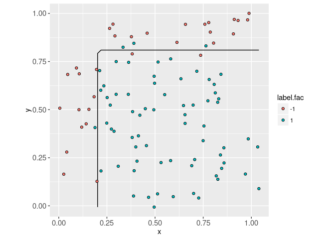
Forward and back propagation in linear model
To implement the gradient descent algorithm for learning neural network model parameters, we will use a simple auto-grad system. Auto-grad is the idea that the neural network model structure should be defined once, and that structure should be used to derive both the forward (prediction) and backward (gradient) propagation computations. Below we use a simple auto-grad system where each node in the computation graph is represented by an R environment (a mutable data structure, necessary so that the gradients are back-propagated to all the model parameters). The function below is a constructor for the most basic building block of the auto-grad system, a node in the computation graph:
new_node <- function(value, gradient=NULL, ...){
  node <- new.env()
  node$value <- value
  node$parent.list <- list(...)
  node$backward <- function(){
    grad.list <- gradient(node)
    for(parent.name in names(grad.list)){
      parent.node <- node$parent.list[[parent.name]]
      parent.node$grad <- grad.list[[parent.name]]
      parent.node$backward()
    }
  }
  node
}
The code in the function above starts by creating a new environment, then populates it with three objects:
valueis a matrix computed by forward propagation at this node in the computation graph.parent.listis a list of parent nodes, each of which is used to computevalue.backwardis a function which should be called by the user on the final/loss node in the computation graph. It callsgradient, which should compute the gradient of the loss with respect to the parent nodes, which are stored in thegradattribute in each corresponding parent node, before recursively callingbackwardon each parent node.
The simplest kind of node is an initial node, defined by the code below,
initial_node <- function(mat){
  new_node(mat, gradient=function(...)list())
}
The code above says that an initial node simply stores the input matrix mat as the value, and has a gradient method that does nothing (because initial nodes in the computation graph have no parents for which gradients could be computed). The code below defines mm, a node in the computation graph which represents a matrix multiplication,
mm <- function(feature.node, weight.node)new_node(
  cbind(1, feature.node$value) %*% weight.node$value,
  features=feature.node,
  weights=weight.node,
  gradient=function(node)list(
    features=node$grad %*% t(weight.node$value),
    weights=t(cbind(1, feature.node$value)) %*% node$grad))
The mm definition above assumes that there is a weight node with the same number of rows as the number of columns (plus one for intercept) in the feature node. The forward/value and gradient computations use matrix multiplication. For instance, we can use mm as follows to define a simple linear model,
feature.node <- initial_node(features.noisy[is.set.list$subtrain,])
weight.node <- initial_node(rep(0, ncol(features.noisy)+1))
linear.pred.node <- mm(feature.node, weight.node)
str(linear.pred.node$value)
## num [1:50, 1] 0 0 0 0 0 0 0 0 0 0 ...It can be seen in the code above that the mm function returns a node representing predicted values, one for each row in the feature matrix. To use the gradient features we need a loss function, which in the case of binary classification is the logistic (cross-entropy) loss,
log_loss <- function(pred.node, label.node)new_node(
  mean(log(1+exp(-label.node$value*pred.node$value))),
  pred=pred.node,
  label=label.node,
  gradient=function(...)list(
    pred=-label.node$value/(
      1+exp(label.node$value*pred.node$value)
    )/length(label.node$value)))
The code above defines the logistic loss and gradient, assuming the label is either -1 or 1, and the prediction is a real number (not necessarily between 0 and 1, maybe negative). The code below creates nodes for the labels and loss,
label.node <- initial_node(label.vec[is.set.list$subtrain])
loss.node <- log_loss(linear.pred.node, label.node)
loss.node$value
## [1] 0.6931472Now that we have computed the loss, we can compute the gradient of the loss with respect to the weights, which is used to perform the updates during learning. Remember that we should now call backward (on the subtrain loss), which should eventually store the gradient as weight.node$grad. Below we first verify that it has not yet been computed, then we compute it:
weight.node$grad## NULLloss.node$backward()
weight.node$grad## [,1]
## [1,] -0.16000000
## [2,] -0.10511619
## [3,] -0.02447615Note that since loss.node contains recursive back-references to its parent nodes (including predictions and weights), the backward call above is able to conveniently compute and store weight.node$grad, the gradient of the loss with respect to the weight parameters. The gradient is the direction of steepest ascent, meaning the direction weights could be modified to maximize the loss. Because we want to minimize the loss, the learning algorithm performs updates in the negative gradient direction, of steepest descent.
(descent.direction <- -weight.node$grad)## [,1]
## [1,] 0.16000000
## [2,] 0.10511619
## [3,] 0.02447615In gradient descent for this linear model, we update the weight vector in this direction. Each update to the weight vector is referred to as an iteration or step. A small step in this direction is guaranteed to decrease the loss, but too small of a step will not make much progress toward minimizing the loss. It is unknown how far in this direction is best, so we typically need to search over a grid of step sizes (aka learning rates). Or we can perform a line search, which means making the following plot of loss as a function of step size, then choosing the step size with minimal loss.
(line.search.dt <- data.table(step.size=seq(0, 10, l=101))[, .(
  loss=log_loss(mm(
    feature.node,
    initial_node(weight.node$value+step.size*descent.direction)
  ), label.node)$value
), by=step.size])
## step.size loss
## <num> <num>
## 1: 0.0 0.6931472
## 2: 0.1 0.6894865
## 3: 0.2 0.6859542
## 4: 0.3 0.6825501
## 5: 0.4 0.6792743
## ---
## 97: 9.6 0.8333305
## 98: 9.7 0.8385249
## 99: 9.8 0.8437642
## 100: 9.9 0.8490474
## 101: 10.0 0.8543739line.search.min <- line.search.dt[which.min(loss)]
ggplot()+
geom_line(aes(
step.size, loss),
data=line.search.dt)+
geom_point(aes(
step.size, loss),
data=line.search.min)+
geom_text(aes(
step.size, loss, label=sprintf(
"min loss=%f at step size=%.1f",
loss, step.size)),
data=line.search.min,
size=4,
hjust=0,
vjust=1.5)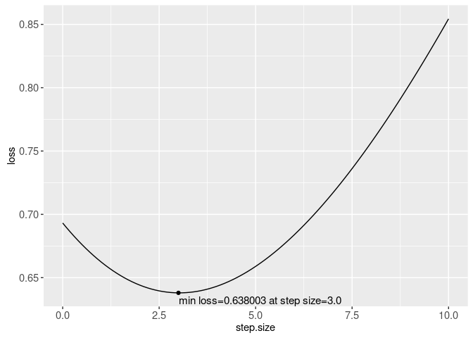
The plot above shows that the min loss occurs at a step size of about 3, which means that the line search would choose that step size for this gradient descent parameter update/iteration, before re-computing the gradient in the next iteration.
Neural network learning
Defining a linear model in the previous section was relatively simple, because there is only one weight matrix parameter (actually, a weight vector, with the same number of elements as the number of columns/features, plus one for an intercept). In contrast, a neural network has more than one weight matrix parameter to learn. We initialize these weights as nodes in the code below,
new_weight_node_list <- function(units.per.layer, intercept=TRUE){
  weight.node.list <- list()
  for(layer.i in seq(1, length(units.per.layer)-1)){
    input.units <- units.per.layer[[layer.i]]+intercept
    output.units <- units.per.layer[[layer.i+1]]
    weight.mat <- matrix(
      rnorm(input.units*output.units), input.units, output.units)
    weight.node.list[[layer.i]] <- initial_node(weight.mat)
  }
  weight.node.list
}
(units.per.layer <- c(ncol(features.noisy), 40, 1))
## [1] 2 40 1(weight.node.list <- new_weight_node_list(units.per.layer))## [[1]]
## <environment: 0x6cf4638>
##
## [[2]]
## <environment: 0x6cf5b00>lapply(weight.node.list, function(node)dim(node$value))## [[1]]
## [1] 3 40
##
## [[2]]
## [1] 41 1The output above shows that there is a single layer with 40 hidden units in the neural network, meaning there are two weight matrices to learn. Each of these weight matrices is used to predict the units in a given layer, from the units in the previous layer. In order to learn a prediction function which is a non-linear function of the features, each layer except for the last must have a non-linear activation function, applied element-wise to the units after matrix multiplication. For example, a common and efficient non-linear activation function is the ReLU (Rectified Linear Units), which is implemented below,
relu <- function(before.node)new_node(
  ifelse(before.node$value < 0, 0, before.node$value),
  before=before.node,
  gradient=function(node)list(
    before=ifelse(before.node$value < 0, 0, node$grad)))
hidden.before.act <- mm(feature.node, weight.node.list[[1]])
str(hidden.before.act$value)
## num [1:50, 1:40] 1.62 3.67 2.34 2.42 1.57 ...hidden.before.act$value[1:5,1:5]## [,1] [,2] [,3] [,4] [,5]
## [1,] 1.617099 -0.31485515 0.8687167 0.5969050 -0.5717334
## [2,] 3.665478 -0.08953216 1.1884750 0.7686507 -0.7655569
## [3,] 2.335856 -1.53696561 1.1271410 0.4960481 -1.2771119
## [4,] 2.418533 -0.61750628 1.0377415 0.6157081 -0.8390015
## [5,] 1.571396 1.26836784 0.6830969 0.7897418 0.2105804hidden.after.act <- relu(hidden.before.act)
hidden.after.act$value[1:5,1:5]## [,1] [,2] [,3] [,4] [,5]
## [1,] 1.617099 0.000000 0.8687167 0.5969050 0.0000000
## [2,] 3.665478 0.000000 1.1884750 0.7686507 0.0000000
## [3,] 2.335856 0.000000 1.1271410 0.4960481 0.0000000
## [4,] 2.418533 0.000000 1.0377415 0.6157081 0.0000000
## [5,] 1.571396 1.268368 0.6830969 0.7897418 0.2105804Note in the output above how the ReLU activation sets negative values to zero, and keeps positive values the same:
(relu.dt <- data.table(
  input=seq(-5, 5, l=101)
)[, output := relu(initial_node(input))$value][])
## input output
## <num> <num>
## 1: -5.0 0.0
## 2: -4.9 0.0
## 3: -4.8 0.0
## 4: -4.7 0.0
## 5: -4.6 0.0
## ---
## 97: 4.6 4.6
## 98: 4.7 4.7
## 99: 4.8 4.8
## 100: 4.9 4.9
## 101: 5.0 5.0ggplot()+
ggtitle("ReLU activation is non-linear")+
geom_line(aes(
input, output),
data=relu.dt)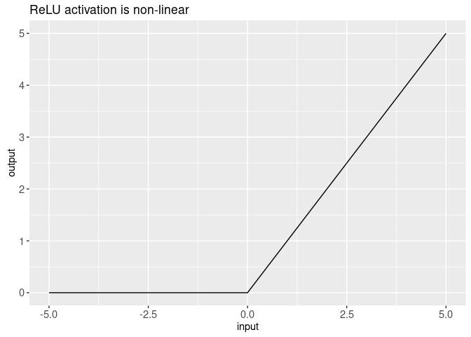
Finally, the last node that we need to implement our neural network is a node for predictions, computed via the for loop over weight nodes in the function below,
pred_node <- function(set.features){
  feature.node <- initial_node(set.features)
  for(layer.i in seq_along(weight.node.list)){
    weight.node <- weight.node.list[[layer.i]]
    before.node <- mm(feature.node, weight.node)
    feature.node <- if(layer.i < length(weight.node.list)){
      relu(before.node)
    }else{
      before.node
    }
  }
  feature.node
}
nn.pred.node <- pred_node(features.noisy[is.set.list$subtrain,])
str(nn.pred.node$value)
## num [1:50, 1] 3.85 6.42 2.14 3.54 8.18 ...The pred_node function is also useful for computing predictions on the grid of features, which will be useful later for visualizing the learned function,
grid.mat <- grid.dt[, cbind(V1,V2)]
nn.grid.node <- pred_node(grid.mat)
str(nn.grid.node$value)
## num [1:900, 1] 1.74 2.09 2.43 2.78 3.12 ...The code below combines all of the pieces above into a gradient descent learning algorithm. The hyper-parameters are the constant step size, and the maximum number of iterations.
step.size <- 0.5
max.iterations <- 1000
units.per.layer <- c(ncol(features.noisy), 40, 1)
loss.dt.list <- list()
err.dt.list <- list()
pred.dt.list <- list()
set.seed(10)
weight.node.list <- new_weight_node_list(units.per.layer)
for(iteration in 1:max.iterations){
  loss.node.list <- list()
  for(set in names(is.set.list)){
    is.set <- is.set.list[[set]]
    set.label.node <- initial_node(label.vec[is.set])
    set.features <- features.noisy[is.set,]
    set.pred.node <- pred_node(set.features)
    set.loss.node <- log_loss(set.pred.node, set.label.node)
    loss.node.list[[set]] <- set.loss.node
    set.pred.num <- ifelse(set.pred.node$value<0, -1, 1)
    is.error <- set.pred.num != set.label.node$value
    err.dt.list[[paste(iteration, set)]] <- data.table(
      iteration, set,
      set.features,
      label=set.label.node$value,
      pred.num=as.numeric(set.pred.num))
    loss.dt.list[[paste(iteration, set)]] <- data.table(
      iteration, set,
      mean.log.loss=set.loss.node$value,
      error.percent=100*mean(is.error))
  }
  grid.node <- pred_node(grid.mat)
  pred.dt.list[[paste(iteration)]] <- data.table(
    iteration,
    grid.dt,
    pred=as.numeric(grid.node$value))
  loss.node.list$subtrain$backward()#<-back-prop.
  for(layer.i in seq_along(weight.node.list)){
    weight.node <- weight.node.list[[layer.i]]
    weight.node$value <- #learning/param updates:
      weight.node$value-step.size*weight.node$grad
  }
}
loss.dt <- rbindlist(loss.dt.list)
err.dt <- rbindlist(err.dt.list)
pred.dt <- rbindlist(pred.dt.list)
loss.tall <- melt(loss.dt, measure=c("mean.log.loss", "error.percent"))
loss.tall[, log10.iteration := log10(iteration)]
min.dt <- loss.tall[
, .SD[which.min(value)], by=.(set, variable)]
ggplot()+
  facet_grid(variable ~ ., scales="free")+
  scale_y_continuous("")+
  geom_line(aes(
    iteration, value, color=set),
    data=loss.tall)+
  geom_point(aes(
    iteration, value, fill=set),
    shape=21,
    color="black",
    data=min.dt)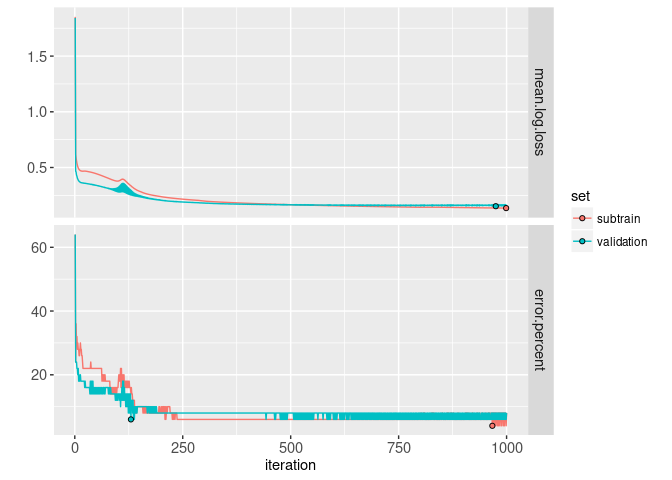
In the code above we saved loss and predictions for all of the iterations of gradient descent, but in the code below we visualize only some of them, due to limited space:
some <- function(DT)DT[iteration%in%c(1,5,10,50,100)]
err.dt[, prediction := ifelse(label==pred.num, "correct", "error")]
iteration.contours <- pred.dt[
, get_boundary(pred), by=.(iteration)]
some.loss <- some(loss.dt)
pred.dt[, norm.pred := pred/max(abs(pred)), by=.(iteration)]
some.pred <- some(pred.dt)
some.err <- some(err.dt)
some.contours <- some.pred[
, get_boundary(pred), by=.(iteration)]
ggplot()+
  facet_grid(set ~ iteration, labeller="label_both")+
  geom_tile(aes(
    V1, V2, fill=norm.pred),
    color=NA,
    data=some.pred)+
  geom_path(aes(
    x, y, group=contour.i),
    color="grey50",
    data=some.contours)+
  scale_fill_gradient2()+
  geom_point(aes(
    V1, V2, color=prediction, fill=label/2),
    shape=21,
    size=2,
    data=some.err)+
  scale_color_manual(
    values=c(correct="white", error="black"))+
  coord_equal()+
  scale_y_continuous(breaks=seq(0,1,by=0.5))+
  scale_x_continuous(breaks=seq(0,1,by=0.5))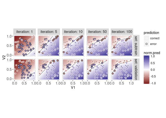
From the plot above we can see that as the number of iterations increases, the predictions get more accurate. Finally, we conclude with an interactive plot where you can click the loss plot to select an iteration of gradient descent, for which the corresponding decision boundary is shown on the predictions plot.
n.subtrain <- sum(is.set.list$subtrain)
loss.dt[, n.set := ifelse(set=="subtrain", n.subtrain, sim.row-n.subtrain)]
loss.dt[, error.count := n.set*error.percent/100]
it.by <- 10
some <- function(DT)DT[iteration%in%as.integer(seq(1,max.iterations,by=it.by))]
animint(
  title="Neural network vs linear model",
  out.dir="neural-networks-sim",
  loss=ggplot()+
    ggtitle("Loss/error curves, click to select model/iteration")+
    theme_bw()+
    theme_animint(width=600, height=350)+
    theme(panel.margin=grid::unit(1, "lines"))+
    facet_grid(variable ~ ., scales="free")+
    scale_y_continuous("")+
    scale_x_continuous(
      "Iteration/epoch of learning, with gradient computed on subtrain set")+
    geom_line(aes(
      iteration, value, color=set, group=set),
      data=loss.tall)+
    geom_point(aes(
      iteration, value, fill=set),
      shape=21,
      color="black",
      data=min.dt)+
    geom_tallrect(aes(
      xmin=iteration-it.by/2,
      xmax=iteration+it.by/2),
      alpha=0.5,
      clickSelects="iteration",
      data=some(loss.tall[set=="subtrain"])),
  data=ggplot()+
    ggtitle("Learned function at selected model/iteration")+
    theme_bw()+
    theme_animint(width=600)+
    facet_grid(. ~ set, labeller="label_both")+
    geom_tile(aes(
      V1, V2, fill=norm.pred),
      color=NA,
      showSelected="iteration",
      data=some(pred.dt))+
    geom_text(aes(
      0.5, 1.1, label=paste0(
        "loss=", round(mean.log.loss, 4),
        ", ", error.count, "/", n.set,
        " errors=", error.percent, "%")),
      showSelected="iteration",
      data=loss.dt)+
    geom_path(aes(
      x, y, group=contour.i),
      showSelected="iteration",
      color="grey50",
      data=some(iteration.contours))+
    geom_point(aes(
      V1, V2, fill=label/2, color=prediction),
      showSelected=c("iteration", "set"),
      size=4,
      data=some(err.dt))+
    scale_fill_gradient2(
      "Class/Score")+
    scale_color_manual(
      values=c(correct="white", error="black"))+
    scale_x_continuous(
      "Input/Feature 1")+
    scale_y_continuous(
      "Input/Feature 2")+
    coord_equal())
Chapter summary and exercises
Exercises:
- Add animation over the number of iterations.
- Add smooth transitions when changing the selected number of iterations.
- Add a for loop over random seeds (or cross-validation folds) in the data splitting step, and create a visualization that shows how that affects the results.
- Add a for loop over random seeds at the weight matrix initialization step, and create a visualization that shows how that affects the results.
- Compute results for another neural network architecture (and/or linear model, by adding a for loop over different values of
units.per.layer). Add another plot or facet which allows selecting the neural network architecture, and allows easy comparison of the min validation loss between models (for example, add facet columns to loss plot, and add horizontal lines to emphasize min loss). - Modify the learning algorithm to use line search rather than constant step size, and then create a visualization which compares the two approaches in terms of min validation loss.
Next, Chapter 99 explains some R programming idioms that are generally useful for interactive data visualization design.
