Chapter 12, Support Vector Machines
This goal of this chapter is to create an interactive data visualization that explains the Support Vector Machine, a machine learning model for binary classification.
Chapter summary:
- We begin by simulating some data for binary classification in two dimensions, and making some static plots.
- In the second section, we make an interactive data visualization to show how the linear Support Vector Machine decision boundary changes as a function of the cost hyper-parameter.
- In the last section, we make an interactive data visualization to show how the decision boundary of the polynomial kernel Support Vector Machine changes as a function of the two hyper-parameters (cost and degree).
Generate and plot some data
We begin by generating two input features, x1 and x2.
library(data.table)
N <- 50
set.seed(1)
getInput <- function(){
  c(#rnorm(N, sd=0.3),
    runif(N, -1, 1),
    runif(N, -1, 1)
    )
}
data.dt <- data.table(
  x1=getInput(),
  x2=getInput())
library(animint2)
ggplot()+
  geom_point(aes(
    x1, x2),
    data=data.dt)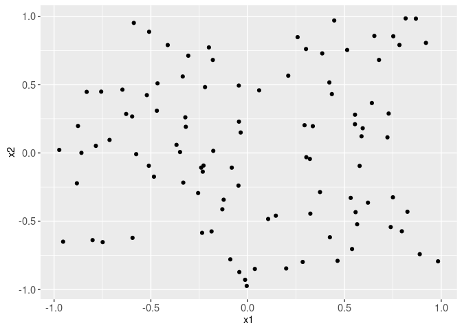
The plot below shows the same data, after computing two additional input features (the squares of the original two inputs).
data.dt[, let(
  x1.sq = x1^2,
  x2.sq = x2^2)][]
## x1 x2 x1.sq x2.sq
## <num> <num> <num> <num>
## 1: -0.468982674 0.3094478562 2.199447e-01 9.575798e-02
## 2: -0.255752201 -0.2936054561 6.540919e-02 8.620416e-02
## 3: 0.145706727 -0.4594797082 2.123045e-02 2.111216e-01
## 4: 0.816415580 0.9853681223 6.665344e-01 9.709503e-01
## 5: -0.596636138 0.2669865289 3.559747e-01 7.128181e-02
## 6: 0.796779370 -0.5735837296 6.348574e-01 3.289983e-01
## 7: 0.889350537 -0.7412553038 7.909444e-01 5.494594e-01
## 8: 0.321595585 -0.0437639314 1.034237e-01 1.915282e-03
## 9: 0.258228088 0.8481489397 6.668175e-02 7.193566e-01
## 10: -0.876427459 0.1975219343 7.681251e-01 3.901491e-02
## 11: -0.588050850 0.9523413898 3.458038e-01 9.069541e-01
## 12: -0.646886495 0.4635850238 4.184621e-01 2.149111e-01
## 13: 0.374045693 -0.2865461758 1.399102e-01 8.210871e-02
## 14: -0.231792564 -0.1370526189 5.372779e-02 1.878342e-02
## 15: 0.539682840 -0.7035768786 2.912576e-01 4.950204e-01
## 16: -0.004601516 -0.9738448490 2.117395e-05 9.483738e-01
## 17: 0.435237017 0.4311321322 1.894313e-01 1.858749e-01
## 18: 0.983812190 -0.7936315285 9.678864e-01 6.298510e-01
## 19: -0.239929641 -0.1074313028 5.756623e-02 1.154148e-02
## 20: 0.554890443 0.2802020903 3.079034e-01 7.851321e-02
## 21: 0.869410462 0.9836772401 7.558746e-01 9.676209e-01
## 22: -0.575714957 -0.0088128443 3.314477e-01 7.766622e-05
## 23: 0.303347532 -0.0313009513 9.201973e-02 9.797495e-04
## 24: -0.748889808 -0.6531153303 5.608359e-01 4.265596e-01
## 25: -0.465558663 0.5096418890 2.167449e-01 2.597349e-01
## 26: -0.227771815 -0.0922090216 5.188000e-02 8.502504e-03
## 27: -0.973219334 0.0223395675 9.471559e-01 4.990563e-04
## 28: -0.235224086 -0.5849097734 5.533037e-02 3.421194e-01
## 29: 0.739381691 -0.5426837145 5.466853e-01 2.945056e-01
## 30: -0.319302007 0.1914239926 1.019538e-01 3.664314e-02
## 31: -0.035839769 0.1497443966 1.284489e-03 2.242338e-02
## 32: 0.199131651 -0.8458712394 3.965341e-02 7.154982e-01
## 33: -0.012917386 -0.9289188408 1.668589e-04 8.628902e-01
## 34: -0.627564797 0.2855909844 3.938376e-01 8.156221e-02
## 35: 0.654746637 0.8572303993 4.286932e-01 7.348440e-01
## 36: 0.336933476 0.1961848447 1.135242e-01 3.848849e-02
## 37: 0.588479721 0.1218014960 3.463084e-01 1.483560e-02
## 38: -0.784112748 0.0520554478 6.148328e-01 2.709770e-03
## 39: 0.447421892 0.9701904478 2.001863e-01 9.412695e-01
## 40: -0.177451141 0.0152836447 3.148891e-02 2.335898e-04
## 41: 0.641892588 0.3655761573 4.120261e-01 1.336459e-01
## 42: 0.294120388 0.2030824353 8.650680e-02 4.124248e-02
## 43: 0.565865525 -0.5222626445 3.202038e-01 2.727583e-01
## 44: 0.106072623 -0.4836681467 1.125140e-02 2.339349e-01
## 45: 0.059439160 0.4586192467 3.533014e-03 2.103316e-01
## 46: 0.578712463 -0.0948583372 3.349081e-01 8.998104e-03
## 47: -0.953337595 -0.6497464632 9.088526e-01 4.221705e-01
## 48: -0.045539870 0.4933965392 2.073880e-03 2.434401e-01
## 49: 0.464627477 -0.7900247192 2.158787e-01 6.241391e-01
## 50: 0.385463113 0.7290898981 1.485818e-01 5.315721e-01
## 51: -0.044760756 0.2292899434 2.003525e-03 5.257388e-02
## 52: 0.722418954 0.1143190777 5.218891e-01 1.306885e-02
## 53: -0.123805786 -0.3424453619 1.532787e-02 1.172688e-01
## 54: -0.510405446 -0.0937371091 2.605137e-01 8.786646e-03
## 55: -0.858641906 0.0008819452 7.372659e-01 7.778274e-07
## 56: -0.801067680 -0.6382672777 6.417094e-01 4.073851e-01
## 57: -0.367456586 0.0592612056 1.350243e-01 3.511890e-03
## 58: 0.037268526 -0.8494485086 1.388943e-03 7.215628e-01
## 59: 0.324010153 -0.4444881347 1.049826e-01 1.975697e-01
## 60: -0.186339626 -0.5746009615 3.472246e-02 3.301663e-01
## 61: 0.825751849 -0.4304190380 6.818661e-01 1.852605e-01
## 62: -0.412793254 0.7901882059 1.703983e-01 6.243974e-01
## 63: -0.081868547 -0.1075293534 6.702459e-03 1.156256e-02
## 64: -0.335210652 0.5599697796 1.123662e-01 3.135662e-01
## 65: 0.301740934 0.7612380697 9.104759e-02 5.794834e-01
## 66: -0.483966439 -0.1737515810 2.342235e-01 3.018961e-02
## 67: -0.042909503 -0.8723830390 1.841225e-03 7.610522e-01
## 68: 0.532621341 -0.3290250166 2.836855e-01 1.082575e-01
## 69: -0.831506171 0.4474518932 6.914025e-01 2.002132e-01
## 70: 0.750642660 -0.3247693330 5.634644e-01 1.054751e-01
## 71: -0.321854124 0.2608282450 1.035901e-01 6.803137e-02
## 72: 0.678880700 0.6812291080 4.608790e-01 4.640731e-01
## 73: -0.306633022 0.7122633294 9.402381e-02 5.073191e-01
## 74: -0.332450138 -0.2172814379 1.105231e-01 4.721122e-02
## 75: -0.047297510 -0.2390122288 2.237054e-03 5.712685e-02
## 76: 0.784396672 0.7908908520 6.152781e-01 6.255083e-01
## 77: 0.728678941 0.2886315258 5.309730e-01 8.330816e-02
## 78: -0.220020913 0.4821572974 4.840920e-02 2.324757e-01
## 79: 0.554641398 0.2106068931 3.076271e-01 4.435526e-02
## 80: 0.921235994 0.8061632230 8.486758e-01 6.498991e-01
## 81: -0.130681030 -0.4125396898 1.707753e-02 1.701890e-01
## 82: 0.425029357 -0.6174797802 1.806500e-01 3.812813e-01
## 83: -0.200011262 0.7729018866 4.000451e-02 5.973773e-01
## 84: -0.349295696 0.0066789715 1.220075e-01 4.460866e-05
## 85: 0.514174296 0.7541150860 2.643752e-01 5.686896e-01
## 86: -0.594615490 -0.6216127551 3.535676e-01 3.864024e-01
## 87: 0.422242445 0.5162061048 1.782887e-01 2.664687e-01
## 88: -0.756616158 0.4489977853 5.724680e-01 2.015990e-01
## 89: -0.509022972 0.8874496366 2.591044e-01 7.875669e-01
## 90: -0.713391241 0.0952931740 5.089271e-01 9.080789e-03
## 91: -0.520741170 0.4234877354 2.711714e-01 1.793419e-01
## 92: -0.882131245 -0.2221898003 7.781555e-01 4.936831e-02
## 93: 0.284576517 -0.7982537476 8.098379e-02 6.372090e-01
## 94: 0.752538425 0.8546041772 5.663141e-01 7.303483e-01
## 95: 0.557829355 -0.4335349994 3.111736e-01 1.879526e-01
## 96: 0.594617652 0.1811463176 3.535702e-01 3.281399e-02
## 97: -0.089451093 -0.7792787901 8.001498e-03 6.072754e-01
## 98: -0.179831836 0.6810140642 3.233949e-02 4.637802e-01
## 99: 0.621740486 -0.3640726311 3.865612e-01 1.325489e-01
## 100: 0.209866581 0.5657026740 4.404398e-02 3.200195e-01
## x1 x2 x1.sq x2.sqggplot()+
geom_point(aes(
x1.sq, x2.sq),
data=data.dt)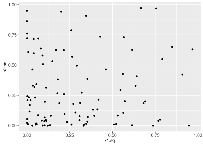
In our simulation, we assume that the output score f is a linear function of x1.sq, and ignores x2.sq. The plot below visualizes the output scores using the point fill aesthetic.
data.dt[, f := x1.sq]
true.decision.boundary <- 0.2
ggplot()+
  theme_bw()+
  scale_fill_gradient2(midpoint=true.decision.boundary)+
  geom_point(aes(
    x1.sq, x2.sq, fill=f),
    shape=21,
    color="grey",
    data=data.dt)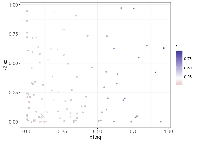
In particular, we assume that the label y is negative (-1) if x1.sq + noise < threshold, and positive (1) otherwise. The plot below visualizes the scores and labels, as a function of the input feature x1. It also shows the true score function in black. Of course, we would not be able to make this visualization with real data (only the labels are known in real data, not the scores).
data.dt[
, f.noise := f+rnorm(N, 0, 0.2)
][
, y.num := ifelse(f.noise<true.decision.boundary, -1, 1)
][
, y := factor(y.num)
]
table(data.dt$y)
##
## -1 1
## 56 44scores <- data.table(x1=seq(-1, 1, l=101))[
, x1.sq := x1^2
][
, f := x1.sq ]
x1.boundaries <- data.table(boundary=c(1, -1)*sqrt(true.decision.boundary))
ggplot()+
scale_y_continuous(breaks=seq(0, 1, by=0.2))+
geom_vline(aes(xintercept=boundary), color="grey50", data=x1.boundaries)+
geom_line(aes(x1, f), data=scores)+
geom_point(aes(
x1, f.noise, color=y),
shape=21,
fill=NA,
data=data.dt)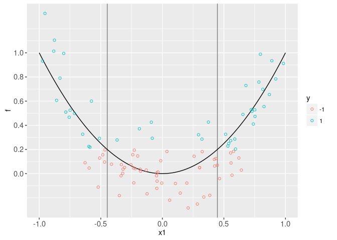
The plot below shows the scores and labels, as a function of the squared feature x1.sq. It is clear that the score function that we want to learn is linear in x1.sq.
x1sq.boundary <- data.table(boundary=true.decision.boundary)
ggplot()+
  scale_y_continuous(breaks=seq(0, 1, by=0.2))+
  scale_x_continuous(breaks=seq(0, 1, by=0.2))+
  geom_vline(aes(
    xintercept=boundary),
    color="grey50",
    data=x1sq.boundary)+
  geom_line(aes(x1.sq, f), data=scores)+
  geom_point(aes(
    x1.sq, f.noise, color=y),
    shape=21,
    fill=NA,
    data=data.dt)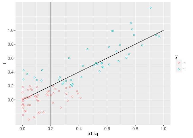
Next, we visualize the labels in the two-dimensional squared feature space. It is clear that the decision boundary is linear in this space.
ggplot()+
  scale_y_continuous(breaks=seq(0, 1, by=0.2))+
  scale_x_continuous(breaks=seq(0, 1, by=0.2))+
  geom_vline(aes(
    xintercept=boundary),
    color="grey50",
    data=x1sq.boundary)+
  geom_point(aes(
    x1.sq, x2.sq, color=y),
    shape=21,
    fill=NA,
    data=data.dt)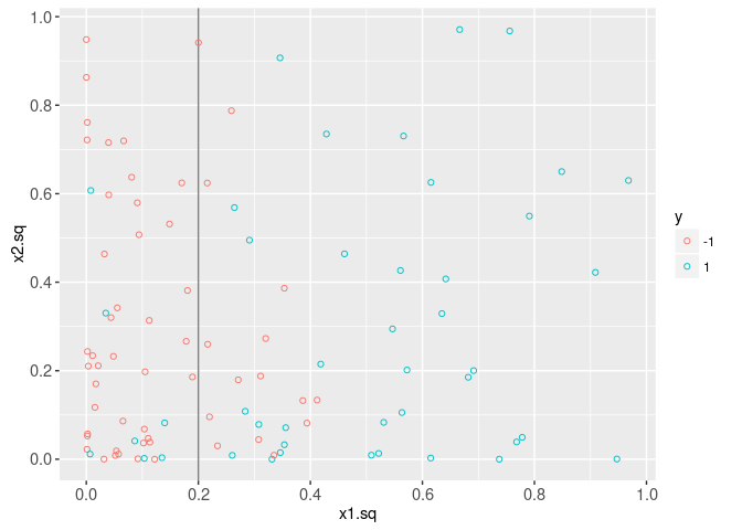
The plot below shows the input feature space (x1 and x2). It is clear that the decision boundary is non-linear in x1.
ggplot()+
  scale_y_continuous(breaks=seq(-1, 1, by=0.2))+
  scale_x_continuous(breaks=seq(-1, 1, by=0.2))+
  geom_vline(aes(
    xintercept=boundary),
    color="grey50",
    data=x1.boundaries)+
  geom_point(aes(
    x1, x2, color=y),
    shape=21,
    fill=NA,
    data=data.dt)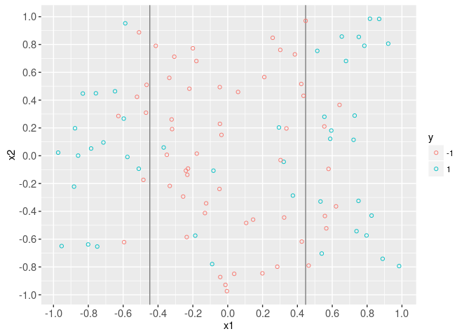
The animint below uses clickSelects to show which points in the input and squared space correspond. We just need to create an data.i variable that has a unique ID for each data point.
data.dt[, data.i := 1:.N]
YVAR <- function(dt, y.var){
  dt$y.var <- factor(y.var, c("x2", "x2.sq", "f"))
  dt
}
animint(
  input=ggplot()+
    ggtitle("input feature space")+
    theme_bw()+
    theme(panel.margin=grid::unit(0, "lines"))+
    facet_grid(y.var ~ ., scales="free")+
    scale_x_continuous(breaks=seq(-1, 1, by=0.2))+
    ylab("")+
    guides(color="none")+
    geom_vline(aes(
      xintercept=boundary),
      color="grey50",
      data=x1.boundaries)+
    geom_point(aes(
      x1, x2, color=y),
      clickSelects="data.i",
      size=4,
      alpha=0.7,
      data=YVAR(data.dt, "x2"))+
    geom_line(aes(
      x1, f),
      data=YVAR(scores, "f"))+
    geom_point(aes(
      x1, f.noise, color=y),
      clickSelects="data.i",
      size=4,
      alpha=0.7,
      data=YVAR(data.dt, "f")),
  square=ggplot()+
    ggtitle("squared feature space")+
    theme_bw()+
    theme(panel.margin=grid::unit(0, "lines"))+
    facet_grid(y.var ~ ., scales="free")+
    ylab("")+
    scale_x_continuous(breaks=seq(0, 1, by=0.2))+
    geom_vline(aes(
      xintercept=boundary),
      color="grey50",
      data=x1sq.boundary)+
    geom_point(aes(
      x1.sq, x2.sq, color=y),
      clickSelects="data.i",
      size=4,
      alpha=0.7,
      data=YVAR(data.dt, "x2.sq"))+
    geom_line(aes(
      x1.sq, f),
      data=YVAR(scores, "f"))+
    geom_point(aes(
      x1.sq, f.noise, color=y),
      clickSelects="data.i",
      size=4,
      alpha=0.7,
      data=YVAR(data.dt, "f")))
Note how we used two multi-panel plots with the addColumn then facet idiom, rather than creating four separate plots. This emphasizes the fact that some plots/facets have a common x1 or x1.sq axis. Note that we also hid the color legend in the first plot, since it is sufficient to just have one color legend.
Linear SVM
train.i <- 1:N
data.dt[
, set := "test"
][
  train.i, set := "train"
]
table(data.dt$set)
##
## test train
## 50 50train.dt <- data.dt[set=="train",]
ggplot()+
theme_bw()+
theme(panel.margin=grid::unit(0, "lines"))+
facet_grid(set ~ .)+
geom_vline(aes(
xintercept=boundary),
color="grey50",
data=x1.boundaries)+
scale_y_continuous(breaks=seq(-1, 1, by=0.2))+
scale_x_continuous(breaks=seq(-1, 1, by=0.2))+
geom_point(aes(
x1, x2, color=y),
data=data.dt)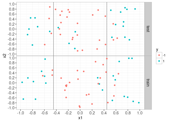
We begin by fitting a linear SVM to the train data in the squared feature space, and visualizing the true labels y along with the predicted labels pred.y.
library(kernlab)
squared.mat <- train.dt[, cbind(x1.sq, x2.sq)]
y.vec <- train.dt$y
fit <- ksvm(squared.mat, y.vec, kernel="vanilladot")
## Setting default kernel parameterstrain.dt$pred.y <- predict(fit)
ggplot()+
geom_point(aes(
x1.sq, x2.sq, color=pred.y, fill=y),
shape=21,
size=4,
stroke=2,
data=train.dt)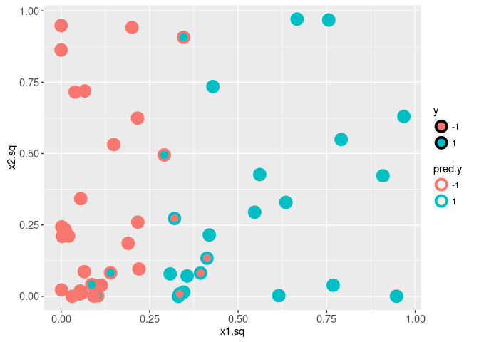
It is clear from the plot above that there are several mis-classified train data points. In the plot below we visualize the decision boundary and margin.
predF <- function(fit, X){
  fit.sc <- scaling(fit)$x.scale
  if(is.null(fit.sc)){
    fit.sc <- list(
      "scaled:center"=c(0,0),
      "scaled:scale"=c(1,1))
  }
  mu <- fit.sc[["scaled:center"]]
  sigma <- fit.sc[["scaled:scale"]]
  X.sc <- scale(X, mu, sigma)
  kernelMult(
    kernelf(fit),
    X.sc,
    xmatrix(fit)[[1]],
    coef(fit)[[1]])-b(fit)
}
xsq.vec <- seq(0, 1, l=41)
grid.sq.dt <- data.table(expand.grid(
  x1.sq=xsq.vec,
  x2.sq=xsq.vec
))[
, pred.f := predF(fit, cbind(x1.sq, x2.sq))]
train.dt[, train.error := ifelse(y==pred.y, "correct", "error")]
ggplot()+
  theme_bw()+
  scale_color_manual(values=c(error="black", correct=NA))+
  geom_point(aes(
    x1.sq, x2.sq, fill=y, color=train.error),
    shape=21,
    stroke=1,
    size=4,
    data=train.dt)+
  geom_vline(aes(
    xintercept=boundary), color="grey50",
    data=x1sq.boundary)+
  geom_contour(aes(
    x1.sq, x2.sq, z=pred.f),
    breaks=0,
    color="black",
    data=grid.sq.dt)+
  geom_contour(aes(
    x1.sq, x2.sq, z=pred.f),
    breaks=c(-1, 1),
    color="black",
    linetype="dashed",
    data=grid.sq.dt)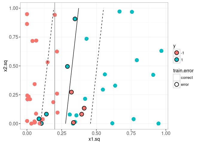
The plot above shows the true decision boundary using a grey vline. It also uses geom_contour to display the decision boundary (solid black line, predicted score 0) and the margin (dashed black line, predicted score -1 and 1). Since the decision boundary and margin are linear in this space, we can also use geom_abline to display them. To do that we need to do some math, and work out the equations for the slope and intercepts of those lines (as a function of the learned bias b(fit) and weight.vec, as well as the scale parameters mu and sigma).
## The equation of the margin lines is x2 = m2 + s2/w2[c+b+w1*m1/s1]
## -s2*w1/(w2*s1)*x1 for c=1 and -1. x is input feature, m is mean, s
## is scale, w is learned weight.
fit.sc <- scaling(fit)$x.scale
if(is.null(fit.sc)){
  fit.sc <- list(
    "scaled:center"=c(0,0),
    "scaled:scale"=c(1,1))
}
mu <- fit.sc[["scaled:center"]]
sigma <- fit.sc[["scaled:scale"]]
weight.vec <- colSums(xmatrix(fit)[[1]]*coef(fit)[[1]])
predF.linear <- function(fit, X){
  X.sc <- scale(X, mu, sigma)
  X.sc %*% weight.vec - b(fit)
}
abline.dt <- data.table(
  y=factor(c(-1,0,1)),
  boundary=c("margin", "decision", "margin"),
  intercept=mu[2]+sigma[2]/weight.vec[2]*(
    c(-1, 0, 1)+b(fit)+weight.vec[1]*mu[1]/sigma[1]),
  slope=-weight.vec[1]*sigma[2]/(weight.vec[2]*sigma[1]))
ggplot()+
  theme_bw()+
  scale_linetype_manual(values=c(margin="dashed", decision="solid"))+
  geom_abline(aes(
    slope=slope, intercept=intercept, linetype=boundary),
    color="green",
    size=1,
    data=abline.dt)+
  geom_point(aes(
    x1.sq, x2.sq, color=y),
    shape=21,
    fill=NA,
    size=4,
    data=train.dt)+
  geom_contour(aes(
    x1.sq, x2.sq, z=pred.f),
    breaks=0,
    color="black",
    data=grid.sq.dt)+
  geom_contour(aes(
    x1.sq, x2.sq, z=pred.f),
    breaks=c(-1, 1),
    color="black",
    linetype="dashed",
    data=grid.sq.dt)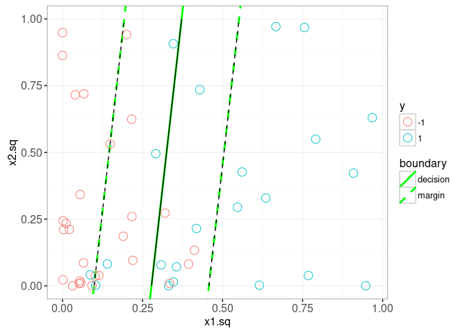
The plot above confirms that our computation of the slope and intercepts (green lines) agrees with the contours (black lines). In the plot below, we show the learned alpha coefficients, and add a geom_segment to visualize the slack.
train.dt[, alpha := 0]
train.row.vec <- as.integer(rownames(xmatrix(fit)[[1]]))
train.dt[train.row.vec, alpha := kernlab::alpha(fit)[[1]] ]
train.dt[, status := ifelse(
  alpha==0, "alpha=0",
  ifelse(alpha==1, "alpha=C", "0<alpha<C"))]
slack.slope <- weight.vec[2]*sigma[1]/(weight.vec[1]*sigma[2])
slack.dt <- train.dt[alpha==1,]
slack.join <- abline.dt[slack.dt, on=list(y)]
slack.join[, x1.sq.margin := (
  x2.sq-slack.slope*x1.sq-intercept)/(slope-slack.slope)]
slack.join[, x2.sq.margin := slope*x1.sq.margin + intercept]
sv.colors <- c(
  "alpha=0"="white",
  "0<alpha<C"="black",
  "alpha=C"="grey")
ggplot()+
  theme_bw()+
  scale_linetype_manual(values=c(margin="dashed", decision="solid"))+
  geom_vline(aes(
    xintercept=boundary), color="violet",
    data=x1sq.boundary)+
  geom_abline(aes(
    slope=slope, intercept=intercept, linetype=boundary),
    size=1,
    data=abline.dt)+
  geom_segment(aes(
    x1.sq, x2.sq,
    xend=x1.sq.margin, yend=x2.sq.margin),
    color="grey",
    data=slack.join)+
  scale_fill_manual(values=sv.colors, breaks=names(sv.colors))+
  geom_point(aes(
    x1.sq, x2.sq, color=y, fill=status),
    shape=21,
    size=4,
    data=train.dt)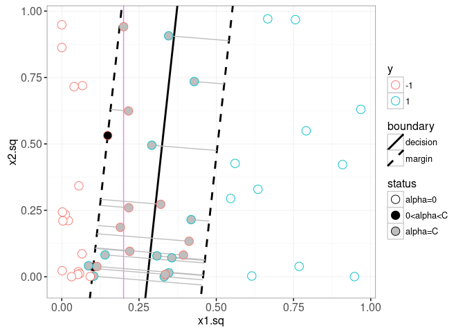
The plot above shows the slack in grey segments, and the decision and margin lines in black. The Bayes decision boundary is shown in the background as a vertical violet line. The support vectors are the points with non-zero alpha coefficients. Black filled support vectors are on the margin, and grey support vectors are on the wrong side of the margin (and have non-zero slack). The plot below shows the model that was learned in the original feature space,
n.grid <- 41
x.vec <- seq(-1, 1, l=n.grid)
grid.dt <- data.table(expand.grid(
  x1=x.vec,
  x2=x.vec))
getBoundaryDF <- function(score.vec, level.vec=c(-1, 0, 1)){
  stopifnot(length(score.vec) == n.grid * n.grid)
  several.paths <- contourLines(
    x.vec, x.vec,
    matrix(score.vec, n.grid, n.grid),
    levels=level.vec)
  contour.list <- list()
  for(path.i in seq_along(several.paths)){
    contour.list[[path.i]] <- with(several.paths[[path.i]], data.table(
      path.i,
      level.num=as.numeric(level),
      level.fac=factor(level, level.vec),
      boundary=ifelse(level==0, "decision", "margin"),
      x1=x, x2=y))
  }
  do.call(rbind, contour.list)
}
grid.dt[, pred.f := predF(fit, cbind(x1^2, x2^2))]
boundaries <- grid.dt[, getBoundaryDF(pred.f)]
ggplot()+
  scale_linetype_manual(values=c(margin="dashed", decision="solid"))+
  geom_vline(aes(
    xintercept=boundary),
    color="violet",
    data=x1.boundaries)+
  geom_path(aes(
    x1, x2, group=path.i, linetype=boundary),
    size=1,
    data=boundaries)+
  scale_fill_manual(values=sv.colors, breaks=names(sv.colors))+
  scale_size_manual(values=c(correct=2, error=4))+
  geom_point(aes(
    x1, x2, color=y,
    size=train.error,
    fill=status),
    shape=21,
    data=train.dt)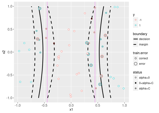
The goal below will be to make an animint that shows how the decision boundary, margin, and slack change as a function of the cost parameter.
modelInfo.list <- list()
predictions.list <- list()
slackSegs.list <- list()
modelLines.list <- list()
inputBoundaries.list <- list()
setErrors.list <- list()
cost.by <- 0.2
for(cost.param in round(10^seq(-1, 1, by=cost.by),1)){
  fit <- ksvm(
    squared.mat, y.vec, kernel="vanilladot", scaled=FALSE, C=cost.param)
  fit.sc <- scaling(fit)$x.scale
  if(is.null(fit.sc)){
    fit.sc <- list(
      "scaled:center"=c(0,0),
      "scaled:scale"=c(1,1))
  }
  mu <- fit.sc[["scaled:center"]]
  sigma <- fit.sc[["scaled:scale"]]
  weight.vec <- colSums(xmatrix(fit)[[1]]*coef(fit)[[1]])
  grid.sq.dt[, pred.f := predF(fit, cbind(x1.sq, x2.sq))]
  data.dt[, pred.y := predict(fit, cbind(x1.sq, x2.sq))]
  one.error <- data.dt[, list(errors=sum(y!=pred.y)), by=set]
  setErrors.list[[paste(cost.param)]] <- data.table(
    cost.param, one.error)
  train.dt[, pred.f := predF(fit, cbind(x1^2, x2^2))]
  grid.dt[, pred.f := predF(fit, cbind(x1^2, x2^2))]
  boundaries <- getBoundaryDF(grid.dt$pred.f)
  inputBoundaries.list[[paste(cost.param)]] <- data.table(
    cost.param, boundaries)
  train.dt$alpha <- 0
  train.row.vec <- as.integer(rownames(xmatrix(fit)[[1]]))
  train.dt[train.row.vec, alpha := kernlab::alpha(fit)[[1]] ]
  train.dt[, status := ifelse(
    alpha==0, "alpha=0",
    ifelse(alpha==cost.param, "alpha=C", "0<alpha<C"))]
  ## The equation of the margin lines is x2 = m2 + s2/w2[c+b+w1*m1/s1]
  ## -s2*w1/(w2*s1)*x1 for c=1 and -1. x is input feature, m is mean, s
  ## is scale, w is learned weight.
  slack.slope <- weight.vec[2]*sigma[1]/(weight.vec[1]*sigma[2])
  abline.dt <- data.table(
    y=factor(c(-1,0,1)),
    boundary=c("margin", "decision", "margin"),
    intercept=mu[2]+sigma[2]/weight.vec[2]*(
      c(-1, 0, 1)+b(fit)+weight.vec[1]*mu[1]/sigma[1]),
    slope=-weight.vec[1]*sigma[2]/(weight.vec[2]*sigma[1]))
  slack.dt <- train.dt[alpha==cost.param]
  slack.join <- abline.dt[slack.dt, on=list(y)]
  slack.join[, x1.sq.margin := (
    x2.sq-slack.slope*x1.sq-intercept)/(slope-slack.slope)]
  slack.join[, x2.sq.margin := slope*x1.sq.margin + intercept]
  norm.weights <- as.numeric(weight.vec %*% weight.vec)
  modelInfo.list[[paste(cost.param)]] <- data.table(
    cost.param,
    slack=slack.join[, sum(1-pred.f*y.num)],
    norm=norm.weights,
    margin=2/sqrt(norm.weights))
  predictions.list[[paste(cost.param)]] <- data.table(
    cost.param, train.dt)
  slackSegs.list[[paste(cost.param)]] <- data.table(
    cost.param, slack.join)
  modelLines.list[[paste(cost.param)]] <- data.table(
    cost.param, abline.dt)
}
## Setting default kernel parameters
## Setting default kernel parameters
## Setting default kernel parameters
## Setting default kernel parameters
## Setting default kernel parameters
## Setting default kernel parameters
## Setting default kernel parameters
## Setting default kernel parameters
## Setting default kernel parameters
## Setting default kernel parameters
## Setting default kernel parametersinputBoundaries <- do.call(rbind, inputBoundaries.list)
predictions <- do.call(rbind, predictions.list)
slackSegs <- do.call(rbind, slackSegs.list)
modelLines <- do.call(rbind, modelLines.list)
modelInfo <- do.call(rbind, modelInfo.list)
setErrors <- do.call(rbind, setErrors.list)
modelInfo.tall <- melt(modelInfo, id.vars="cost.param")
grid.sq.dt$boundary <- "true"
setErrors$variable <- "errors"
inputBoundaries[, boundary := ifelse(level.num==0, "decision", "margin")]
slackSegs$boundary <- "margin"
set.label.select <- data.table(
cost.param=range(setErrors$cost.param),
set=c("test", "train"),
hjust=c(1, 0))
set.labels <- setErrors[set.label.select, on=list(cost.param, set)]
animint(
selectModel=ggplot()+
ggtitle("select regularization parameter")+
geom_tallrect(aes(
xmin=log10(cost.param)-cost.by/2,
xmax=log10(cost.param)+cost.by/2),
clickSelects="cost.param",
alpha=0.5,
data=modelInfo)+
theme_bw()+
facet_grid(variable ~ ., scales="free")+
geom_line(aes(
log10(cost.param), errors,
group=set, color=set),
data=setErrors)+
geom_text(aes(
log10(cost.param), errors-1, label=set,
hjust=hjust,
color=set),
data=set.labels)+
guides(color="none")+
geom_line(aes(
log10(cost.param), log10(value)),
data=modelInfo.tall),
inputSpace=ggplot()+
ggtitle("Input space features")+
scale_fill_manual(values=sv.colors, breaks=names(sv.colors))+
geom_vline(aes(
xintercept=boundary),
color="violet",
data=x1.boundaries)+
guides(color="none", fill="none", linetype="none")+
scale_linetype_manual(values=c(
"-1"="dashed",
"0"="solid",
"1"="dashed"))+
geom_path(aes(
x1, x2,
group=path.i,
linetype=level.fac),
showSelected=c("boundary", "cost.param"),
color="black",
data=inputBoundaries)+
geom_point(aes(
x1, x2, fill=status),
showSelected=c("status", "y", "data.i", "cost.param"),
size=5,
color="grey",
data=predictions)+
geom_point(aes(
x1, x2, color=y, fill=status),
showSelected=c("cost.param", "status", "y"),
clickSelects="data.i",
size=3,
data=predictions),
kernelSpace=ggplot()+
ggtitle("Kernel space features")+
geom_vline(aes(
xintercept=boundary), color="violet",
data=x1sq.boundary)+
##coord_cartesian(xlim=c(0, 1), ylim=c(0, 1))+
geom_abline(aes(
slope=slope, intercept=intercept, linetype=boundary),
showSelected="cost.param",
color="black",
data=modelLines)+
scale_linetype_manual(values=c(
decision="solid",
margin="dashed",
true="solid"))+
geom_point(aes(
x1.sq, x2.sq, fill=status),
showSelected=c("data.i", "cost.param"),
size=5,
color="grey",
data=predictions)+
geom_point(aes(
x1.sq, x2.sq, color=y, fill=status),
clickSelects="data.i",
showSelected="cost.param",
size=3,
data=predictions)+
scale_fill_manual(values=sv.colors, breaks=names(sv.colors))+
geom_segment(aes(
x1.sq, x2.sq,
xend=x1.sq.margin, yend=x2.sq.margin),
showSelected=c("cost.param", "boundary"),
color="grey",
data=slackSegs))
Non-linear polynomial kernel SVM
In the previous section we fit a linear kernel in the squared feature space, which resulted in learning a function which is non-linear in terms of the original feature space. In this section we directly fit a non-linear polynomial kernel in the original space.
predictions.list <- list()
inputBoundaries.list <- list()
setErrors.list <- list()
cost.by <- 0.2
orig.mat <- train.dt[, cbind(x1, x2)]
for(cost.param in 10^seq(-1, 3, by=cost.by)){
  for(degree.num in seq(1, 6, by=1)){
    k <- polydot(degree.num, offset=0)
    fit <- ksvm(
      orig.mat, y.vec, kernel=k, scaled=FALSE, C=cost.param)
    grid.dt[, pred.f := predF(fit, cbind(x1, x2))]
    grid.dt[, pred.y := predict(fit, cbind(x1, x2))]
    grid.dt[, stopifnot(sign(pred.f) == pred.y)]
    data.dt[, pred.y := predict(fit, cbind(x1, x2))]
    one.error <- data.dt[, list(errors=sum(y != pred.y)), by=set]
    setErrors.list[[paste(cost.param, degree.num)]] <- data.table(
      cost.param, degree.num, one.error)
    boundaries <- getBoundaryDF(grid.dt$pred.f)
    if(is.data.frame(boundaries) && nrow(boundaries)){
      cost.deg <- paste(cost.param, degree.num)
      inputBoundaries.list[[cost.deg]] <- data.table(
        cost.param, degree.num, boundaries)
    }
    train.dt[, alpha := 0]
    train.row.vec <- as.integer(rownames(xmatrix(fit)[[1]]))
    train.dt[train.row.vec, alpha := kernlab::alpha(fit)[[1]] ]
    train.dt[, status := ifelse(
      alpha==0, "alpha=0",
      ifelse(alpha==cost.param, "alpha=C", "0<alpha<C"))]
    predictions.list[[paste(cost.param, degree.num)]] <- data.table(
      cost.param, degree.num, train.dt)
  }
}
inputBoundaries <- do.call(rbind, inputBoundaries.list)
predictions <- do.call(rbind, predictions.list)
setErrors <- do.call(rbind, setErrors.list)

testErrors <- setErrors[set=="test"]
testErrors$select <- "degree"
setErrors$select <- "cost"

animint(
  selectModel=ggplot()+
    ggtitle("select hyper parameters")+
    geom_tallrect(aes(
      xmin=log10(cost.param)-cost.by/2,
      xmax=log10(cost.param)+cost.by/2),
      clickSelects="cost.param",
      alpha=0.5,
      data=setErrors[degree.num==1 & set=="train",])+
    theme_bw()+
    theme(panel.margin=grid::unit(0, "lines"))+
    facet_grid(select ~ ., scales="free")+
    ylab("")+
    geom_line(aes(
      log10(cost.param), errors,
      key=set,
      group=set,
      color=set),
      showSelected="degree.num",
      data=setErrors)+
    scale_fill_gradient("TestErrors", low="white", high="red")+
    geom_tile(aes(
      log10(cost.param), degree.num, fill=errors),
      clickSelects="degree.num",
      data=testErrors),
  inputSpace=ggplot()+
    theme_bw()+
    ggtitle("Input space features")+
    scale_fill_manual(values=sv.colors, breaks=names(sv.colors))+
    geom_vline(aes(
      xintercept=boundary),
      color="violet",
      data=x1.boundaries)+
    scale_linetype_manual(values=c(
      margin="dashed",
      decision="solid"))+
    geom_path(aes(
      x1, x2,
      group=path.i,
      linetype=boundary),
      showSelected=c("degree.num", "cost.param"),
      color="black",
      data=inputBoundaries)+
    geom_point(aes(
      x1, x2, color=y, fill=status),
      showSelected=c("cost.param", "degree.num"),
      size=3,
      data=predictions))
Chapter summary and exercises
We used ggplots to visualize the Support Vector Machine model for binary classification. We used animint and interactivity to show how the SVM decision boundary changes as a function of the model hyper-parameters.
Exercises:
- Use
rbfdotas the kernel function. Compute train and test error, then add a new panel to the “select hyper parameters” plot. - By default ggplot2 uses the same two colors for the y and set legends, which could be confusing. Change the colors in one of the two legends so that they are different.
- Use
colorandcolor_offparameters to change the appearance of thegeom_tilewhen selected or not, as explained in Chapter 6, section Specifying how selection state is displayed.
Next, Chapter 13 explains how to visualize the Poisson regression model.
