Chapter 9, Montreal bikes data viz
In this chapter we will explore several data visualizations of the Montreal bike data set.
Chapter outline:
- We begin with some static data visualizations.
- We create an interactive visualization of accident frequency over time.
- We create a interactive data viz with four plots, showing monthly accident trends, daily details, and a map of counter locations.
Static figures
We begin by loading the montreal.bikes data set, which is not available in the CRAN release of animint2, in order to save space on CRAN. Therefore to access this data set, you will need to install animint2 from GitHub:
tryCatch({
  data(montreal.bikes, package="animint2")
}, warning=function(w){
  devtools::install_github("tdhock/animint2")
})
We begin by examining the accidents data table.
library(animint2)
data(montreal.bikes) #only present if installed from github
Sys.setlocale(locale="en_US.UTF-8")
## [1] "LC_CTYPE=en_US.UTF-8;LC_NUMERIC=C;LC_TIME=en_US.UTF-8;LC_COLLATE=en_US.UTF-8;LC_MONETARY=en_US.UTF-8;LC_MESSAGES=fr_FR.UTF-8;LC_PAPER=fr_FR.UTF-8;LC_NAME=C;LC_ADDRESS=C;LC_TELEPHONE=C;LC_MEASUREMENT=fr_FR.UTF-8;LC_IDENTIFICATION=C"if(! "Brébeuf" %in% montreal.bikes$counter.counts$location){
Encoding(levels(montreal.bikes$counter.counts$location)) <- "UTF-8"
print(table(montreal.bikes$counter.counts$location))
}
library(data.table)
accidents.dt <- data.table(montreal.bikes$accidents)
str(accidents.dt)## Classes 'data.table' and 'data.frame': 5595 obs. of 12 variables:
## $ date.str : chr "2012-01-02" "2012-01-05" "2012-01-09" "2012-01-10" ...
## $ time.str : chr "18:35" "21:50" "21:15" "15:40" ...
## $ deaths : int 0 0 0 0 0 0 0 1 0 0 ...
## $ people.severely.injured: int 0 0 0 0 0 0 0 0 0 0 ...
## $ people.slightly.injured: int 1 1 1 1 1 1 1 0 1 1 ...
## $ street.number : int NA NA NA NA NA 2330 NA NA 4160 NA ...
## $ street : chr "ST JEAN BAPTISTE O" "FOSTER" "ROSEMONT" "ST ANTOINE" ...
## $ cross.street : chr "AV ROULEAU" "JANELLE" "DES ERABLES" "MANSFIELD" ...
## $ location.int : int 32 34 NA 32 32 34 32 32 33 31 ...
## $ position.int : int 6 6 6 6 6 6 6 6 6 5 ...
## $ position : chr "Voie de circulation" "Voie de circulation" "Voie de circulation" "Voie de circulation" ...
## $ location : chr "En intersection (moins de 5 mètres)" "Entre intersections (100 mètres et +)" NA "En intersection (moins de 5 mètres)" ...
## - attr(*, ".internal.selfref")=<externalptr>Each accident has data about its date, time, location, and counts of death and slight/severe injury. Some of the values are in French (e.g. position Voie de circulation, location En intersection, etc).
We calculate the time period of the accidents below.
(accidents.dt[
, date.POSIXct := as.POSIXct(strptime(date.str, "%Y-%m-%d"))
][
, month.str := strftime(date.POSIXct, "%Y-%m")
][])
## date.str time.str deaths people.severely.injured
## <char> <char> <int> <int>
## 1: 2012-01-02 18:35 0 0
## 2: 2012-01-05 21:50 0 0
## 3: 2012-01-09 21:15 0 0
## 4: 2012-01-10 15:40 0 0
## 5: 2012-01-10 0:15 0 0
## ---
## 5591: 2014-12-19 12:22 0 0
## 5592: 2014-12-19 19:50 0 0
## 5593: 2014-12-26 19:56 0 0
## 5594: 2014-12-27 12:35 0 0
## 5595: 2014-12-30 11:55 0 0
## people.slightly.injured street.number street cross.street
## <int> <int> <char> <char>
## 1: 1 NA ST JEAN BAPTISTE O AV ROULEAU
## 2: 1 NA FOSTER JANELLE
## 3: 1 NA ROSEMONT DES ERABLES
## 4: 1 NA ST ANTOINE MANSFIELD
## 5: 1 NA TASCHEREAU ANGELE
## ---
## 5591: 1 NA COTE DES NEIGES DES PINS
## 5592: 1 NA BOUTHILLIER N FRONTENAC
## 5593: 1 NA BD DU SEMINAIRE N ST GEORGES
## 5594: 1 NA CH DES PATRIOTES 1RE RUE
## 5595: 1 14965 PIERREFONDS BD JACQUES BIZARD
## location.int position.int position
## <int> <int> <char>
## 1: 32 6 Voie de circulation
## 2: 34 6 Voie de circulation
## 3: NA 6 Voie de circulation
## 4: 32 6 Voie de circulation
## 5: 32 6 Voie de circulation
## ---
## 5591: 32 6 Voie de circulation
## 5592: 32 NA <NA>
## 5593: 32 8 Terre-plein central ou îlot
## 5594: 33 6 Voie de circulation
## 5595: 33 5 Voie cyclable / chaussée désignée
## location date.POSIXct month.str
## <char> <POSc> <char>
## 1: En intersection (moins de 5 mètres) 2012-01-02 2012-01
## 2: Entre intersections (100 mètres et +) 2012-01-05 2012-01
## 3: <NA> 2012-01-09 2012-01
## 4: En intersection (moins de 5 mètres) 2012-01-10 2012-01
## 5: En intersection (moins de 5 mètres) 2012-01-10 2012-01
## ---
## 5591: En intersection (moins de 5 mètres) 2014-12-19 2014-12
## 5592: En intersection (moins de 5 mètres) 2014-12-19 2014-12
## 5593: En intersection (moins de 5 mètres) 2014-12-26 2014-12
## 5594: Près d'une intersection/carrefour giratoire 2014-12-27 2014-12
## 5595: Près d'une intersection/carrefour giratoire 2014-12-30 2014-12range(accidents.dt$month.str)## [1] "2012-01" "2014-12"Below we also compute the range of months for the bike counter data table.
(counts.dt <- data.table(montreal.bikes$counter.counts))## location date count
## <fctr> <POSc> <int>
## 1: Berri 2009-01-01 06:00:00 29
## 2: Berri 2009-01-02 06:00:00 19
## 3: Berri 2009-01-03 06:00:00 24
## 4: Berri 2009-01-04 06:00:00 24
## 5: Berri 2009-01-05 06:00:00 120
## ---
## 13379: Totem_Laurier 2013-09-14 06:00:00 2456
## 13380: Totem_Laurier 2013-09-15 06:00:00 2527
## 13381: Totem_Laurier 2013-09-16 06:00:00 3012
## 13382: Totem_Laurier 2013-09-17 06:00:00 3745
## 13383: Totem_Laurier 2013-09-18 06:00:00 3921counts.dt[, month.str := strftime(date, "%Y-%m")]
range(counts.dt$month.str)## [1] "2009-01" "2013-09"The bike counts are time series data which we visualize below.
counts.dt[, loc.lines := gsub("[- _]", "\n", location)]
ggplot()+
  theme_bw()+
  theme(panel.margin=grid::unit(0, "lines"))+
  facet_grid(loc.lines ~ .)+
  geom_point(aes(
    date, count, color=count==0),
    shape=21,
    data=counts.dt)+
  scale_color_manual(values=c("TRUE"="grey", "FALSE"="black"))
## Warning: Removed 407 rows containing missing values (geom_point).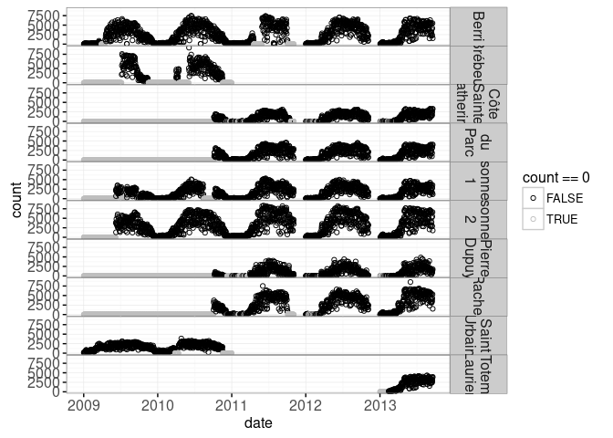
Plotting with geom_point makes it easy to see the difference between zeros and missing values.
We will compute a summary of all accidents per month in this time period, so we first create a data table for each month below. (and make sure to set the locale to C for English month names)
uniq.month.vec <- unique(c(
  accidents.dt$month.str,
  counts.dt$month.str))
one.day <- 60 * 60 * 24
months <- data.table(month.str=uniq.month.vec)[
, month01.str := paste0(month.str, "-01")
][
, month01.POSIXct := as.POSIXct(strptime(month01.str, "%Y-%m-%d"))
][, let(
  next.POSIXct = month01.POSIXct + one.day * 31,
  month.str = strftime(month01.POSIXct, "%B %Y")
)][
, next01.str := paste0(strftime(next.POSIXct, "%Y-%m"), "-01")
][
, next01.POSIXct := as.POSIXct(strptime(next01.str, "%Y-%m-%d"))
]
month.levs <- months[order(month01.POSIXct), month.str]
(months[, month := factor(month.str, month.levs)][])
## month.str month01.str month01.POSIXct next.POSIXct next01.str
## <char> <char> <POSc> <POSc> <char>
## 1: January 2012 2012-01-01 2012-01-01 2012-02-01 00:00:00 2012-02-01
## 2: February 2012 2012-02-01 2012-02-01 2012-03-03 00:00:00 2012-03-01
## 3: March 2012 2012-03-01 2012-03-01 2012-04-01 01:00:00 2012-04-01
## 4: April 2012 2012-04-01 2012-04-01 2012-05-02 00:00:00 2012-05-01
## 5: May 2012 2012-05-01 2012-05-01 2012-06-01 00:00:00 2012-06-01
## 6: June 2012 2012-06-01 2012-06-01 2012-07-02 00:00:00 2012-07-01
## 7: July 2012 2012-07-01 2012-07-01 2012-08-01 00:00:00 2012-08-01
## 8: August 2012 2012-08-01 2012-08-01 2012-09-01 00:00:00 2012-09-01
## 9: September 2012 2012-09-01 2012-09-01 2012-10-02 00:00:00 2012-10-01
## 10: October 2012 2012-10-01 2012-10-01 2012-10-31 23:00:00 2012-10-01
## 11: November 2012 2012-11-01 2012-11-01 2012-12-02 00:00:00 2012-12-01
## 12: December 2012 2012-12-01 2012-12-01 2013-01-01 00:00:00 2013-01-01
## 13: January 2013 2013-01-01 2013-01-01 2013-02-01 00:00:00 2013-02-01
## 14: February 2013 2013-02-01 2013-02-01 2013-03-04 00:00:00 2013-03-01
## 15: March 2013 2013-03-01 2013-03-01 2013-04-01 01:00:00 2013-04-01
## 16: April 2013 2013-04-01 2013-04-01 2013-05-02 00:00:00 2013-05-01
## 17: May 2013 2013-05-01 2013-05-01 2013-06-01 00:00:00 2013-06-01
## 18: June 2013 2013-06-01 2013-06-01 2013-07-02 00:00:00 2013-07-01
## 19: July 2013 2013-07-01 2013-07-01 2013-08-01 00:00:00 2013-08-01
## 20: August 2013 2013-08-01 2013-08-01 2013-09-01 00:00:00 2013-09-01
## 21: September 2013 2013-09-01 2013-09-01 2013-10-02 00:00:00 2013-10-01
## 22: October 2013 2013-10-01 2013-10-01 2013-10-31 23:00:00 2013-10-01
## 23: November 2013 2013-11-01 2013-11-01 2013-12-02 00:00:00 2013-12-01
## 24: December 2013 2013-12-01 2013-12-01 2014-01-01 00:00:00 2014-01-01
## 25: January 2014 2014-01-01 2014-01-01 2014-02-01 00:00:00 2014-02-01
## 26: February 2014 2014-02-01 2014-02-01 2014-03-04 00:00:00 2014-03-01
## 27: March 2014 2014-03-01 2014-03-01 2014-04-01 01:00:00 2014-04-01
## 28: April 2014 2014-04-01 2014-04-01 2014-05-02 00:00:00 2014-05-01
## 29: May 2014 2014-05-01 2014-05-01 2014-06-01 00:00:00 2014-06-01
## 30: June 2014 2014-06-01 2014-06-01 2014-07-02 00:00:00 2014-07-01
## 31: July 2014 2014-07-01 2014-07-01 2014-08-01 00:00:00 2014-08-01
## 32: August 2014 2014-08-01 2014-08-01 2014-09-01 00:00:00 2014-09-01
## 33: September 2014 2014-09-01 2014-09-01 2014-10-02 00:00:00 2014-10-01
## 34: October 2014 2014-10-01 2014-10-01 2014-10-31 23:00:00 2014-10-01
## 35: November 2014 2014-11-01 2014-11-01 2014-12-02 00:00:00 2014-12-01
## 36: December 2014 2014-12-01 2014-12-01 2015-01-01 00:00:00 2015-01-01
## 37: January 2009 2009-01-01 2009-01-01 2009-02-01 00:00:00 2009-02-01
## 38: February 2009 2009-02-01 2009-02-01 2009-03-04 00:00:00 2009-03-01
## 39: March 2009 2009-03-01 2009-03-01 2009-04-01 01:00:00 2009-04-01
## 40: April 2009 2009-04-01 2009-04-01 2009-05-02 00:00:00 2009-05-01
## 41: May 2009 2009-05-01 2009-05-01 2009-06-01 00:00:00 2009-06-01
## 42: June 2009 2009-06-01 2009-06-01 2009-07-02 00:00:00 2009-07-01
## 43: July 2009 2009-07-01 2009-07-01 2009-08-01 00:00:00 2009-08-01
## 44: August 2009 2009-08-01 2009-08-01 2009-09-01 00:00:00 2009-09-01
## 45: September 2009 2009-09-01 2009-09-01 2009-10-02 00:00:00 2009-10-01
## 46: October 2009 2009-10-01 2009-10-01 2009-10-31 23:00:00 2009-10-01
## 47: November 2009 2009-11-01 2009-11-01 2009-12-02 00:00:00 2009-12-01
## 48: December 2009 2009-12-01 2009-12-01 2010-01-01 00:00:00 2010-01-01
## 49: January 2010 2010-01-01 2010-01-01 2010-02-01 00:00:00 2010-02-01
## 50: February 2010 2010-02-01 2010-02-01 2010-03-04 00:00:00 2010-03-01
## 51: March 2010 2010-03-01 2010-03-01 2010-04-01 01:00:00 2010-04-01
## 52: April 2010 2010-04-01 2010-04-01 2010-05-02 00:00:00 2010-05-01
## 53: May 2010 2010-05-01 2010-05-01 2010-06-01 00:00:00 2010-06-01
## 54: June 2010 2010-06-01 2010-06-01 2010-07-02 00:00:00 2010-07-01
## 55: July 2010 2010-07-01 2010-07-01 2010-08-01 00:00:00 2010-08-01
## 56: August 2010 2010-08-01 2010-08-01 2010-09-01 00:00:00 2010-09-01
## 57: September 2010 2010-09-01 2010-09-01 2010-10-02 00:00:00 2010-10-01
## 58: October 2010 2010-10-01 2010-10-01 2010-10-31 23:00:00 2010-10-01
## 59: November 2010 2010-11-01 2010-11-01 2010-12-02 00:00:00 2010-12-01
## 60: December 2010 2010-12-01 2010-12-01 2011-01-01 00:00:00 2011-01-01
## 61: January 2011 2011-01-01 2011-01-01 2011-02-01 00:00:00 2011-02-01
## 62: February 2011 2011-02-01 2011-02-01 2011-03-04 00:00:00 2011-03-01
## 63: March 2011 2011-03-01 2011-03-01 2011-04-01 01:00:00 2011-04-01
## 64: April 2011 2011-04-01 2011-04-01 2011-05-02 00:00:00 2011-05-01
## 65: May 2011 2011-05-01 2011-05-01 2011-06-01 00:00:00 2011-06-01
## 66: June 2011 2011-06-01 2011-06-01 2011-07-02 00:00:00 2011-07-01
## 67: July 2011 2011-07-01 2011-07-01 2011-08-01 00:00:00 2011-08-01
## 68: August 2011 2011-08-01 2011-08-01 2011-09-01 00:00:00 2011-09-01
## 69: September 2011 2011-09-01 2011-09-01 2011-10-02 00:00:00 2011-10-01
## 70: October 2011 2011-10-01 2011-10-01 2011-10-31 23:00:00 2011-10-01
## 71: November 2011 2011-11-01 2011-11-01 2011-12-02 00:00:00 2011-12-01
## 72: December 2011 2011-12-01 2011-12-01 2012-01-01 00:00:00 2012-01-01
## month.str month01.str month01.POSIXct next.POSIXct next01.str
## next01.POSIXct month
## <POSc> <fctr>
## 1: 2012-02-01 January 2012
## 2: 2012-03-01 February 2012
## 3: 2012-04-01 March 2012
## 4: 2012-05-01 April 2012
## 5: 2012-06-01 May 2012
## 6: 2012-07-01 June 2012
## 7: 2012-08-01 July 2012
## 8: 2012-09-01 August 2012
## 9: 2012-10-01 September 2012
## 10: 2012-10-01 October 2012
## 11: 2012-12-01 November 2012
## 12: 2013-01-01 December 2012
## 13: 2013-02-01 January 2013
## 14: 2013-03-01 February 2013
## 15: 2013-04-01 March 2013
## 16: 2013-05-01 April 2013
## 17: 2013-06-01 May 2013
## 18: 2013-07-01 June 2013
## 19: 2013-08-01 July 2013
## 20: 2013-09-01 August 2013
## 21: 2013-10-01 September 2013
## 22: 2013-10-01 October 2013
## 23: 2013-12-01 November 2013
## 24: 2014-01-01 December 2013
## 25: 2014-02-01 January 2014
## 26: 2014-03-01 February 2014
## 27: 2014-04-01 March 2014
## 28: 2014-05-01 April 2014
## 29: 2014-06-01 May 2014
## 30: 2014-07-01 June 2014
## 31: 2014-08-01 July 2014
## 32: 2014-09-01 August 2014
## 33: 2014-10-01 September 2014
## 34: 2014-10-01 October 2014
## 35: 2014-12-01 November 2014
## 36: 2015-01-01 December 2014
## 37: 2009-02-01 January 2009
## 38: 2009-03-01 February 2009
## 39: 2009-04-01 March 2009
## 40: 2009-05-01 April 2009
## 41: 2009-06-01 May 2009
## 42: 2009-07-01 June 2009
## 43: 2009-08-01 July 2009
## 44: 2009-09-01 August 2009
## 45: 2009-10-01 September 2009
## 46: 2009-10-01 October 2009
## 47: 2009-12-01 November 2009
## 48: 2010-01-01 December 2009
## 49: 2010-02-01 January 2010
## 50: 2010-03-01 February 2010
## 51: 2010-04-01 March 2010
## 52: 2010-05-01 April 2010
## 53: 2010-06-01 May 2010
## 54: 2010-07-01 June 2010
## 55: 2010-08-01 July 2010
## 56: 2010-09-01 August 2010
## 57: 2010-10-01 September 2010
## 58: 2010-10-01 October 2010
## 59: 2010-12-01 November 2010
## 60: 2011-01-01 December 2010
## 61: 2011-02-01 January 2011
## 62: 2011-03-01 February 2011
## 63: 2011-04-01 March 2011
## 64: 2011-05-01 April 2011
## 65: 2011-06-01 May 2011
## 66: 2011-07-01 June 2011
## 67: 2011-08-01 July 2011
## 68: 2011-09-01 August 2011
## 69: 2011-10-01 September 2011
## 70: 2011-10-01 October 2011
## 71: 2011-12-01 November 2011
## 72: 2012-01-01 December 2011
## next01.POSIXct monthNote that we created a month column which is a factor ordered by month.levs.
(accidents.dt[
, month.text := strftime(date.POSIXct, "%B %Y")
][
, month := factor(month.text, month.levs)
][
, month.POSIXct := as.POSIXct(strptime(paste0(month.str, "-15"), "%Y-%m-%d"))
][])
## date.str time.str deaths people.severely.injured
## <char> <char> <int> <int>
## 1: 2012-01-02 18:35 0 0
## 2: 2012-01-05 21:50 0 0
## 3: 2012-01-09 21:15 0 0
## 4: 2012-01-10 15:40 0 0
## 5: 2012-01-10 0:15 0 0
## ---
## 5591: 2014-12-19 12:22 0 0
## 5592: 2014-12-19 19:50 0 0
## 5593: 2014-12-26 19:56 0 0
## 5594: 2014-12-27 12:35 0 0
## 5595: 2014-12-30 11:55 0 0
## people.slightly.injured street.number street cross.street
## <int> <int> <char> <char>
## 1: 1 NA ST JEAN BAPTISTE O AV ROULEAU
## 2: 1 NA FOSTER JANELLE
## 3: 1 NA ROSEMONT DES ERABLES
## 4: 1 NA ST ANTOINE MANSFIELD
## 5: 1 NA TASCHEREAU ANGELE
## ---
## 5591: 1 NA COTE DES NEIGES DES PINS
## 5592: 1 NA BOUTHILLIER N FRONTENAC
## 5593: 1 NA BD DU SEMINAIRE N ST GEORGES
## 5594: 1 NA CH DES PATRIOTES 1RE RUE
## 5595: 1 14965 PIERREFONDS BD JACQUES BIZARD
## location.int position.int position
## <int> <int> <char>
## 1: 32 6 Voie de circulation
## 2: 34 6 Voie de circulation
## 3: NA 6 Voie de circulation
## 4: 32 6 Voie de circulation
## 5: 32 6 Voie de circulation
## ---
## 5591: 32 6 Voie de circulation
## 5592: 32 NA <NA>
## 5593: 32 8 Terre-plein central ou îlot
## 5594: 33 6 Voie de circulation
## 5595: 33 5 Voie cyclable / chaussée désignée
## location date.POSIXct month.str
## <char> <POSc> <char>
## 1: En intersection (moins de 5 mètres) 2012-01-02 2012-01
## 2: Entre intersections (100 mètres et +) 2012-01-05 2012-01
## 3: <NA> 2012-01-09 2012-01
## 4: En intersection (moins de 5 mètres) 2012-01-10 2012-01
## 5: En intersection (moins de 5 mètres) 2012-01-10 2012-01
## ---
## 5591: En intersection (moins de 5 mètres) 2014-12-19 2014-12
## 5592: En intersection (moins de 5 mètres) 2014-12-19 2014-12
## 5593: En intersection (moins de 5 mètres) 2014-12-26 2014-12
## 5594: Près d'une intersection/carrefour giratoire 2014-12-27 2014-12
## 5595: Près d'une intersection/carrefour giratoire 2014-12-30 2014-12
## month.text month month.POSIXct
## <char> <fctr> <POSc>
## 1: January 2012 January 2012 2012-01-15
## 2: January 2012 January 2012 2012-01-15
## 3: January 2012 January 2012 2012-01-15
## 4: January 2012 January 2012 2012-01-15
## 5: January 2012 January 2012 2012-01-15
## ---
## 5591: December 2014 December 2014 2014-12-15
## 5592: December 2014 December 2014 2014-12-15
## 5593: December 2014 December 2014 2014-12-15
## 5594: December 2014 December 2014 2014-12-15
## 5595: December 2014 December 2014 2014-12-15stopifnot(!is.na(accidents.dt$month.POSIXct))
(accidents.per.month <- accidents.dt[, list(
total.accidents=.N,
total.people=sum(deaths+people.severely.injured+people.slightly.injured),
deaths=sum(deaths),
people.severely.injured=sum(people.severely.injured),
people.slightly.injured=sum(people.slightly.injured),
next.POSIXct = month.POSIXct + one.day * 30,
month01.str = paste0(strftime(month.POSIXct, "%Y-%m"), "-01")
), by=.(month, month.str, month.text, month.POSIXct)][, let(
month01.POSIXct = as.POSIXct(strptime(month01.str, "%Y-%m-%d")),
next01.str = paste0(strftime(next.POSIXct, "%Y-%m"), "-01")
)][
, next01.POSIXct := as.POSIXct(strptime(next01.str, "%Y-%m-%d"))
][])## month month.str month.text month.POSIXct total.accidents
## <fctr> <char> <char> <POSc> <int>
## 1: January 2012 2012-01 January 2012 2012-01-15 11
## 2: February 2012 2012-02 February 2012 2012-02-15 19
## 3: March 2012 2012-03 March 2012 2012-03-15 76
## 4: April 2012 2012-04 April 2012 2012-04-15 113
## 5: May 2012 2012-05 May 2012 2012-05-15 224
## 6: June 2012 2012-06 June 2012 2012-06-15 276
## 7: July 2012 2012-07 July 2012 2012-07-15 382
## 8: August 2012 2012-08 August 2012 2012-08-15 328
## 9: September 2012 2012-09 September 2012 2012-09-15 280
## 10: October 2012 2012-10 October 2012 2012-10-15 171
## 11: November 2012 2012-11 November 2012 2012-11-15 105
## 12: December 2012 2012-12 December 2012 2012-12-15 17
## 13: January 2013 2013-01 January 2013 2013-01-15 6
## 14: February 2013 2013-02 February 2013 2013-02-15 13
## 15: March 2013 2013-03 March 2013 2013-03-15 28
## 16: April 2013 2013-04 April 2013 2013-04-15 91
## 17: May 2013 2013-05 May 2013 2013-05-15 258
## 18: June 2013 2013-06 June 2013 2013-06-15 286
## 19: July 2013 2013-07 July 2013 2013-07-15 315
## 20: August 2013 2013-08 August 2013 2013-08-15 326
## 21: September 2013 2013-09 September 2013 2013-09-15 268
## 22: October 2013 2013-10 October 2013 2013-10-15 204
## 23: November 2013 2013-11 November 2013 2013-11-15 75
## 24: December 2013 2013-12 December 2013 2013-12-15 15
## 25: January 2014 2014-01 January 2014 2014-01-15 10
## 26: February 2014 2014-02 February 2014 2014-02-15 6
## 27: March 2014 2014-03 March 2014 2014-03-15 12
## 28: April 2014 2014-04 April 2014 2014-04-15 90
## 29: May 2014 2014-05 May 2014 2014-05-15 202
## 30: June 2014 2014-06 June 2014 2014-06-15 269
## 31: July 2014 2014-07 July 2014 2014-07-15 285
## 32: August 2014 2014-08 August 2014 2014-08-15 308
## 33: September 2014 2014-09 September 2014 2014-09-15 279
## 34: October 2014 2014-10 October 2014 2014-10-15 166
## 35: November 2014 2014-11 November 2014 2014-11-15 71
## 36: December 2014 2014-12 December 2014 2014-12-15 10
## month month.str month.text month.POSIXct total.accidents
## total.people deaths people.severely.injured people.slightly.injured
## <int> <int> <int> <int>
## 1: 11 1 0 10
## 2: 20 0 0 20
## 3: 76 0 3 73
## 4: 114 0 5 109
## 5: 228 1 9 218
## 6: 282 3 11 268
## 7: 388 2 15 371
## 8: 338 1 21 316
## 9: 284 2 12 270
## 10: 172 3 7 162
## 11: 105 1 3 101
## 12: 17 0 2 15
## 13: 6 0 0 6
## 14: 14 1 1 12
## 15: 28 1 1 26
## 16: 93 2 6 85
## 17: 268 5 19 244
## 18: 295 0 16 279
## 19: 325 2 21 302
## 20: 333 2 17 314
## 21: 280 4 21 255
## 22: 204 1 13 190
## 23: 76 2 3 71
## 24: 15 0 1 14
## 25: 10 0 0 10
## 26: 6 0 0 6
## 27: 12 0 2 10
## 28: 91 2 6 83
## 29: 211 2 7 202
## 30: 288 0 15 273
## 31: 291 2 20 269
## 32: 315 1 12 302
## 33: 281 3 16 262
## 34: 170 0 8 162
## 35: 72 1 2 69
## 36: 10 0 0 10
## total.people deaths people.severely.injured people.slightly.injured
## next.POSIXct month01.str month01.POSIXct next01.str next01.POSIXct
## <POSc> <char> <POSc> <char> <POSc>
## 1: 2012-02-14 00:00:00 2012-01-01 2012-01-01 2012-02-01 2012-02-01
## 2: 2012-03-16 00:00:00 2012-02-01 2012-02-01 2012-03-01 2012-03-01
## 3: 2012-04-14 01:00:00 2012-03-01 2012-03-01 2012-04-01 2012-04-01
## 4: 2012-05-15 00:00:00 2012-04-01 2012-04-01 2012-05-01 2012-05-01
## 5: 2012-06-14 00:00:00 2012-05-01 2012-05-01 2012-06-01 2012-06-01
## 6: 2012-07-15 00:00:00 2012-06-01 2012-06-01 2012-07-01 2012-07-01
## 7: 2012-08-14 00:00:00 2012-07-01 2012-07-01 2012-08-01 2012-08-01
## 8: 2012-09-14 00:00:00 2012-08-01 2012-08-01 2012-09-01 2012-09-01
## 9: 2012-10-15 00:00:00 2012-09-01 2012-09-01 2012-10-01 2012-10-01
## 10: 2012-11-13 23:00:00 2012-10-01 2012-10-01 2012-11-01 2012-11-01
## 11: 2012-12-15 00:00:00 2012-11-01 2012-11-01 2012-12-01 2012-12-01
## 12: 2013-01-14 00:00:00 2012-12-01 2012-12-01 2013-01-01 2013-01-01
## 13: 2013-02-14 00:00:00 2013-01-01 2013-01-01 2013-02-01 2013-02-01
## 14: 2013-03-17 00:00:00 2013-02-01 2013-02-01 2013-03-01 2013-03-01
## 15: 2013-04-14 01:00:00 2013-03-01 2013-03-01 2013-04-01 2013-04-01
## 16: 2013-05-15 00:00:00 2013-04-01 2013-04-01 2013-05-01 2013-05-01
## 17: 2013-06-14 00:00:00 2013-05-01 2013-05-01 2013-06-01 2013-06-01
## 18: 2013-07-15 00:00:00 2013-06-01 2013-06-01 2013-07-01 2013-07-01
## 19: 2013-08-14 00:00:00 2013-07-01 2013-07-01 2013-08-01 2013-08-01
## 20: 2013-09-14 00:00:00 2013-08-01 2013-08-01 2013-09-01 2013-09-01
## 21: 2013-10-15 00:00:00 2013-09-01 2013-09-01 2013-10-01 2013-10-01
## 22: 2013-11-13 23:00:00 2013-10-01 2013-10-01 2013-11-01 2013-11-01
## 23: 2013-12-15 00:00:00 2013-11-01 2013-11-01 2013-12-01 2013-12-01
## 24: 2014-01-14 00:00:00 2013-12-01 2013-12-01 2014-01-01 2014-01-01
## 25: 2014-02-14 00:00:00 2014-01-01 2014-01-01 2014-02-01 2014-02-01
## 26: 2014-03-17 00:00:00 2014-02-01 2014-02-01 2014-03-01 2014-03-01
## 27: 2014-04-14 01:00:00 2014-03-01 2014-03-01 2014-04-01 2014-04-01
## 28: 2014-05-15 00:00:00 2014-04-01 2014-04-01 2014-05-01 2014-05-01
## 29: 2014-06-14 00:00:00 2014-05-01 2014-05-01 2014-06-01 2014-06-01
## 30: 2014-07-15 00:00:00 2014-06-01 2014-06-01 2014-07-01 2014-07-01
## 31: 2014-08-14 00:00:00 2014-07-01 2014-07-01 2014-08-01 2014-08-01
## 32: 2014-09-14 00:00:00 2014-08-01 2014-08-01 2014-09-01 2014-09-01
## 33: 2014-10-15 00:00:00 2014-09-01 2014-09-01 2014-10-01 2014-10-01
## 34: 2014-11-13 23:00:00 2014-10-01 2014-10-01 2014-11-01 2014-11-01
## 35: 2014-12-15 00:00:00 2014-11-01 2014-11-01 2014-12-01 2014-12-01
## 36: 2015-01-14 00:00:00 2014-12-01 2014-12-01 2015-01-01 2015-01-01
## next.POSIXct month01.str month01.POSIXct next01.str next01.POSIXctWe plot the accidents per month below.
accidents.tall <- melt(
  accidents.per.month,
  measure.vars=c(
    "deaths", "people.severely.injured", "people.slightly.injured"),
  variable.name="severity",
  value.name="people")
severity.colors <- c(
    "people.slightly.injured"="#FEE0D2",#lite red
    "people.severely.injured"="#FB6A4A",
    deaths="#A50F15")#dark red
ggplot()+
  theme_bw()+
  geom_bar(aes(
    month.POSIXct, people, fill=severity),
    stat="identity",
    data=accidents.tall)+
  scale_fill_manual(values=severity.colors)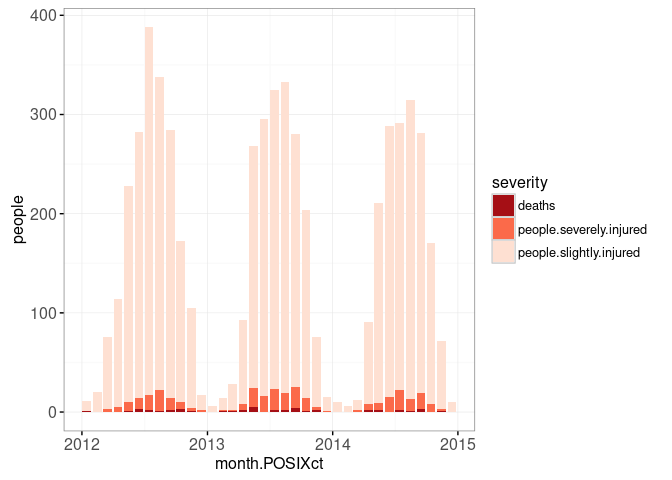
In each accident, there are counts of people who died, along with people who suffered severe and slight injuries. Below we classify the severity of each accident according to the worst outcome among the people affected.
accidents.dt[
, severity.str := fcase(
  0 < deaths, "deaths",
  0 < people.severely.injured, "people.severely.injured",
  default="people.slightly.injured")
][
, severity := factor(severity.str, names(severity.colors))
][
, table(severity)
]
## severity
## people.slightly.injured people.severely.injured deaths
## 5262 289 44The output above shows that accidents with only slight injuries are most frequent, and accidents with at least one death are least frequent. Below we compute counts per month.
(counts.per.month <- counts.dt[, let(
  month.POSIXct = as.POSIXct(strptime(paste0(month.str, "-15"), "%Y-%m-%d")),
  month.text = strftime(date, "%B %Y"),
  day.of.the.month = as.integer(strftime(date, "%d"))
)][
, month := factor(month.text, month.levs)
][, list(
  days=.N,
  mean.per.day=mean(count),
  count=sum(count),
  month01.str = paste0(month.str, "-01")
), by=.(location, month, month.str, month.POSIXct)][
  0 < count
][
, month01.POSIXct := as.POSIXct(strptime(month01.str, "%Y-%m-%d"))
][
, next.POSIXct := month01.POSIXct + one.day * 31
][
, next01.str := paste0(strftime(next.POSIXct, "%Y-%m"), "-01")
][
, next01.POSIXct := as.POSIXct(strptime(next01.str, "%Y-%m-%d"))
][
, days.in.month := as.integer(round(difftime(next01.POSIXct,month01.POSIXct,units="days")))
][])
## location month month.str month.POSIXct days mean.per.day
## <fctr> <fctr> <char> <POSc> <int> <num>
## 1: Berri January 2009 2009-01 2009-01-15 31 100.3226
## 2: Berri February 2009 2009-02 2009-02-15 28 159.6786
## 3: Berri March 2009 2009-03 2009-03-15 31 271.3226
## 4: Berri May 2009 2009-05 2009-05-15 31 2972.8710
## 5: Berri June 2009 2009-06 2009-06-15 30 3909.9333
## ---
## 321: Totem_Laurier May 2013 2013-05 2013-05-15 31 2746.4194
## 322: Totem_Laurier June 2013 2013-06 2013-06-15 30 2828.6000
## 323: Totem_Laurier July 2013 2013-07 2013-07-15 31 3238.3871
## 324: Totem_Laurier August 2013 2013-08 2013-08-15 31 3162.7097
## 325: Totem_Laurier September 2013 2013-09 2013-09-15 18 2888.7778
## count month01.str month01.POSIXct next.POSIXct next01.str
## <int> <char> <POSc> <POSc> <char>
## 1: 3110 2009-01-01 2009-01-01 2009-02-01 00:00:00 2009-02-01
## 2: 4471 2009-02-01 2009-02-01 2009-03-04 00:00:00 2009-03-01
## 3: 8411 2009-03-01 2009-03-01 2009-04-01 01:00:00 2009-04-01
## 4: 92159 2009-05-01 2009-05-01 2009-06-01 00:00:00 2009-06-01
## 5: 117298 2009-06-01 2009-06-01 2009-07-02 00:00:00 2009-07-01
## ---
## 321: 85139 2013-05-01 2013-05-01 2013-06-01 00:00:00 2013-06-01
## 322: 84858 2013-06-01 2013-06-01 2013-07-02 00:00:00 2013-07-01
## 323: 100390 2013-07-01 2013-07-01 2013-08-01 00:00:00 2013-08-01
## 324: 98044 2013-08-01 2013-08-01 2013-09-01 00:00:00 2013-09-01
## 325: 51998 2013-09-01 2013-09-01 2013-10-02 00:00:00 2013-10-01
## next01.POSIXct days.in.month
## <POSc> <int>
## 1: 2009-02-01 31
## 2: 2009-03-01 28
## 3: 2009-04-01 31
## 4: 2009-06-01 31
## 5: 2009-07-01 30
## ---
## 321: 2013-06-01 31
## 322: 2013-07-01 30
## 323: 2013-08-01 31
## 324: 2013-09-01 31
## 325: 2013-10-01 30counts.per.month[days < days.in.month, {
list(location, month, days, days.in.month)
}]## location month days days.in.month
## <fctr> <fctr> <int> <int>
## 1: Berri November 2012 5 30
## 2: Côte-Sainte-Catherine November 2012 5 30
## 3: Maisonneuve 1 November 2012 5 30
## 4: Maisonneuve 2 November 2012 5 30
## 5: du Parc November 2012 5 30
## 6: Pierre-Dupuy November 2012 5 30
## 7: Rachel November 2012 5 30
## 8: Berri September 2013 18 30
## 9: Côte-Sainte-Catherine September 2013 18 30
## 10: Maisonneuve 1 September 2013 18 30
## 11: Maisonneuve 2 September 2013 18 30
## 12: du Parc September 2013 18 30
## 13: Pierre-Dupuy September 2013 18 30
## 14: Rachel September 2013 18 30
## 15: Totem_Laurier September 2013 18 30As shown above, some months do not have observations for all days.
Interactive viz of accident frequency
complete.months <- counts.per.month[days == days.in.month]
month.labels <- counts.per.month[, {
  .SD[which.max(count), ]
}, by=location]
day.labels <- counts.dt[, {
  .SD[which.max(count), ]
}, by=.(location, month)]
(city.wide.cyclists <- counts.per.month[0 < count, list(
  locations=.N,
  count=sum(count),
  month01.str = paste0(month.str, "-01")
), by=.(month, month.str, month.POSIXct)][
, month01.POSIXct := as.POSIXct(strptime(month01.str, "%Y-%m-%d"))
][
, next.POSIXct := month01.POSIXct + one.day * 31
][
, next01.str := paste0(strftime(next.POSIXct, "%Y-%m"), "-01")
][
, next01.POSIXct := as.POSIXct(strptime(next01.str, "%Y-%m-%d"))
][])
## month month.str month.POSIXct locations count month01.str
## <fctr> <char> <POSc> <int> <int> <char>
## 1: January 2009 2009-01 2009-01-15 2 14245 2009-01-01
## 2: February 2009 2009-02 2009-02-15 2 24002 2009-02-01
## 3: March 2009 2009-03 2009-03-15 2 57980 2009-03-01
## 4: May 2009 2009-05 2009-05-15 2 149327 2009-05-01
## 5: June 2009 2009-06 2009-06-15 4 305555 2009-06-01
## 6: July 2009 2009-07 2009-07-15 5 466408 2009-07-01
## 7: August 2009 2009-08 2009-08-15 5 529256 2009-08-01
## 8: September 2009 2009-09 2009-09-15 5 482695 2009-09-01
## 9: October 2009 2009-10 2009-10-15 5 252845 2009-10-01
## 10: November 2009 2009-11 2009-11-15 5 196571 2009-11-01
## 11: December 2009 2009-12 2009-12-15 4 51613 2009-12-01
## 12: April 2009 2009-04 2009-04-15 1 50798 2009-04-01
## 13: January 2010 2010-01 2010-01-15 4 33779 2010-01-01
## 14: February 2010 2010-02 2010-02-15 4 31979 2010-02-01
## 15: March 2010 2010-03 2010-03-15 4 110285 2010-03-01
## 16: April 2010 2010-04 2010-04-15 5 269990 2010-04-01
## 17: May 2010 2010-05 2010-05-15 4 431840 2010-05-01
## 18: June 2010 2010-06 2010-06-15 5 576549 2010-06-01
## 19: July 2010 2010-07 2010-07-15 5 624857 2010-07-01
## 20: August 2010 2010-08 2010-08-15 5 542122 2010-08-01
## 21: September 2010 2010-09 2010-09-15 4 432133 2010-09-01
## 22: October 2010 2010-10 2010-10-15 9 483345 2010-10-01
## 23: November 2010 2010-11 2010-11-15 9 303612 2010-11-01
## 24: December 2010 2010-12 2010-12-15 7 33511 2010-12-01
## 25: January 2011 2011-01 2011-01-15 7 27488 2011-01-01
## 26: February 2011 2011-02 2011-02-15 7 21101 2011-02-01
## 27: March 2011 2011-03 2011-03-15 7 56810 2011-03-01
## 28: April 2011 2011-04 2011-04-15 7 239323 2011-04-01
## 29: May 2011 2011-05 2011-05-15 7 456569 2011-05-01
## 30: June 2011 2011-06 2011-06-15 7 775132 2011-06-01
## 31: July 2011 2011-07 2011-07-15 7 803831 2011-07-01
## 32: August 2011 2011-08 2011-08-15 7 739778 2011-08-01
## 33: September 2011 2011-09 2011-09-15 7 714430 2011-09-01
## 34: October 2011 2011-10 2011-10-15 7 272719 2011-10-01
## 35: January 2012 2012-01 2012-01-15 7 20386 2012-01-01
## 36: February 2012 2012-02 2012-02-15 7 26727 2012-02-01
## 37: March 2012 2012-03 2012-03-15 7 146105 2012-03-01
## 38: April 2012 2012-04 2012-04-15 7 365936 2012-04-01
## 39: May 2012 2012-05 2012-05-15 7 694542 2012-05-01
## 40: June 2012 2012-06 2012-06-15 7 753878 2012-06-01
## 41: July 2012 2012-07 2012-07-15 7 825607 2012-07-01
## 42: August 2012 2012-08 2012-08-15 7 753703 2012-08-01
## 43: September 2012 2012-09 2012-09-15 7 668560 2012-09-01
## 44: October 2012 2012-10 2012-10-15 7 504382 2012-10-01
## 45: November 2012 2012-11 2012-11-15 7 46030 2012-11-01
## 46: January 2013 2013-01 2013-01-15 7 30313 2013-01-01
## 47: February 2013 2013-02 2013-02-15 8 34702 2013-02-01
## 48: March 2013 2013-03 2013-03-15 8 98303 2013-03-01
## 49: April 2013 2013-04 2013-04-15 8 396326 2013-04-01
## 50: May 2013 2013-05 2013-05-15 8 811126 2013-05-01
## 51: June 2013 2013-06 2013-06-15 8 767951 2013-06-01
## 52: July 2013 2013-07 2013-07-15 8 916662 2013-07-01
## 53: August 2013 2013-08 2013-08-15 8 856066 2013-08-01
## 54: September 2013 2013-09 2013-09-15 8 450513 2013-09-01
## month month.str month.POSIXct locations count month01.str
## month01.POSIXct next.POSIXct next01.str next01.POSIXct
## <POSc> <POSc> <char> <POSc>
## 1: 2009-01-01 2009-02-01 00:00:00 2009-02-01 2009-02-01
## 2: 2009-02-01 2009-03-04 00:00:00 2009-03-01 2009-03-01
## 3: 2009-03-01 2009-04-01 01:00:00 2009-04-01 2009-04-01
## 4: 2009-05-01 2009-06-01 00:00:00 2009-06-01 2009-06-01
## 5: 2009-06-01 2009-07-02 00:00:00 2009-07-01 2009-07-01
## 6: 2009-07-01 2009-08-01 00:00:00 2009-08-01 2009-08-01
## 7: 2009-08-01 2009-09-01 00:00:00 2009-09-01 2009-09-01
## 8: 2009-09-01 2009-10-02 00:00:00 2009-10-01 2009-10-01
## 9: 2009-10-01 2009-10-31 23:00:00 2009-10-01 2009-10-01
## 10: 2009-11-01 2009-12-02 00:00:00 2009-12-01 2009-12-01
## 11: 2009-12-01 2010-01-01 00:00:00 2010-01-01 2010-01-01
## 12: 2009-04-01 2009-05-02 00:00:00 2009-05-01 2009-05-01
## 13: 2010-01-01 2010-02-01 00:00:00 2010-02-01 2010-02-01
## 14: 2010-02-01 2010-03-04 00:00:00 2010-03-01 2010-03-01
## 15: 2010-03-01 2010-04-01 01:00:00 2010-04-01 2010-04-01
## 16: 2010-04-01 2010-05-02 00:00:00 2010-05-01 2010-05-01
## 17: 2010-05-01 2010-06-01 00:00:00 2010-06-01 2010-06-01
## 18: 2010-06-01 2010-07-02 00:00:00 2010-07-01 2010-07-01
## 19: 2010-07-01 2010-08-01 00:00:00 2010-08-01 2010-08-01
## 20: 2010-08-01 2010-09-01 00:00:00 2010-09-01 2010-09-01
## 21: 2010-09-01 2010-10-02 00:00:00 2010-10-01 2010-10-01
## 22: 2010-10-01 2010-10-31 23:00:00 2010-10-01 2010-10-01
## 23: 2010-11-01 2010-12-02 00:00:00 2010-12-01 2010-12-01
## 24: 2010-12-01 2011-01-01 00:00:00 2011-01-01 2011-01-01
## 25: 2011-01-01 2011-02-01 00:00:00 2011-02-01 2011-02-01
## 26: 2011-02-01 2011-03-04 00:00:00 2011-03-01 2011-03-01
## 27: 2011-03-01 2011-04-01 01:00:00 2011-04-01 2011-04-01
## 28: 2011-04-01 2011-05-02 00:00:00 2011-05-01 2011-05-01
## 29: 2011-05-01 2011-06-01 00:00:00 2011-06-01 2011-06-01
## 30: 2011-06-01 2011-07-02 00:00:00 2011-07-01 2011-07-01
## 31: 2011-07-01 2011-08-01 00:00:00 2011-08-01 2011-08-01
## 32: 2011-08-01 2011-09-01 00:00:00 2011-09-01 2011-09-01
## 33: 2011-09-01 2011-10-02 00:00:00 2011-10-01 2011-10-01
## 34: 2011-10-01 2011-10-31 23:00:00 2011-10-01 2011-10-01
## 35: 2012-01-01 2012-02-01 00:00:00 2012-02-01 2012-02-01
## 36: 2012-02-01 2012-03-03 00:00:00 2012-03-01 2012-03-01
## 37: 2012-03-01 2012-04-01 01:00:00 2012-04-01 2012-04-01
## 38: 2012-04-01 2012-05-02 00:00:00 2012-05-01 2012-05-01
## 39: 2012-05-01 2012-06-01 00:00:00 2012-06-01 2012-06-01
## 40: 2012-06-01 2012-07-02 00:00:00 2012-07-01 2012-07-01
## 41: 2012-07-01 2012-08-01 00:00:00 2012-08-01 2012-08-01
## 42: 2012-08-01 2012-09-01 00:00:00 2012-09-01 2012-09-01
## 43: 2012-09-01 2012-10-02 00:00:00 2012-10-01 2012-10-01
## 44: 2012-10-01 2012-10-31 23:00:00 2012-10-01 2012-10-01
## 45: 2012-11-01 2012-12-02 00:00:00 2012-12-01 2012-12-01
## 46: 2013-01-01 2013-02-01 00:00:00 2013-02-01 2013-02-01
## 47: 2013-02-01 2013-03-04 00:00:00 2013-03-01 2013-03-01
## 48: 2013-03-01 2013-04-01 01:00:00 2013-04-01 2013-04-01
## 49: 2013-04-01 2013-05-02 00:00:00 2013-05-01 2013-05-01
## 50: 2013-05-01 2013-06-01 00:00:00 2013-06-01 2013-06-01
## 51: 2013-06-01 2013-07-02 00:00:00 2013-07-01 2013-07-01
## 52: 2013-07-01 2013-08-01 00:00:00 2013-08-01 2013-08-01
## 53: 2013-08-01 2013-09-01 00:00:00 2013-09-01 2013-09-01
## 54: 2013-09-01 2013-10-02 00:00:00 2013-10-01 2013-10-01
## month01.POSIXct next.POSIXct next01.str next01.POSIXctmonth.str.vec <- strftime(seq(
strptime("2012-01-15", "%Y-%m-%d"),
strptime("2013-01-15", "%Y-%m-%d"),
by="month"), "%Y-%m")
city.wide.complete <- complete.months[0 < count, list(
locations=.N,
count=sum(count),
month01.str = paste0(month.str, "-01")
), by=.(month, month.str, month.POSIXct)]
setkey(city.wide.complete, month.str)
scatter.cyclists <- city.wide.complete[month.str.vec]
scatter.accidents <- accidents.per.month[scatter.cyclists, on=list(month.str)]
scatter.not.na <- scatter.accidents[!is.na(locations),]
scatter.max <- scatter.not.na[locations==max(locations)]
fit <- lm(total.accidents ~ count - 1, scatter.max)
scatter.max[
, pred.accidents := predict(fit)
][
, mean(total.accidents/count)
]## [1] 0.000428269animint(
regression=ggplot()+
theme_bw()+
ggtitle("Numbers of accidents and cyclists")+
geom_line(aes(
count, pred.accidents),
color="grey",
data=scatter.max)+
geom_point(aes(
count, total.accidents),
shape=1,
clickSelects="month",
size=5,
alpha=0.75,
data=scatter.max)+
ylab("Total bike accidents (all Montreal locations)")+
xlab("Total cyclists (all Montreal locations)"),
timeSeries=ggplot()+
theme_bw()+
ggtitle("Time series of accident frequency")+
xlab("Month")+
geom_point(aes(
month.POSIXct, total.accidents/count),
clickSelects="month",
size=5,
alpha=0.75,
data=scatter.max))
The data viz above shows two data visualizations of city-wide accident frequency over time. The plot on the left shows that the number of accidents grows with the number of cyclists. The plot on the right shows the frequency of accidents over time.
Interactive viz with map and details
The plot below is a dotplot of accidents for each month. Each dot represents one person who got in an accident.
(accidents.cumsum <- accidents.dt[
  order(date.POSIXct, month, severity)
][
, accident.i := seq_along(severity)
, by=.(date.POSIXct, month)
][
, day.of.the.month := as.integer(strftime(date.POSIXct, "%d"))
][])
## date.str time.str deaths people.severely.injured
## <char> <char> <int> <int>
## 1: 2012-01-02 18:35 0 0
## 2: 2012-01-05 21:50 0 0
## 3: 2012-01-09 21:15 0 0
## 4: 2012-01-10 15:40 0 0
## 5: 2012-01-10 0:15 0 0
## ---
## 5591: 2014-12-19 12:22 0 0
## 5592: 2014-12-19 19:50 0 0
## 5593: 2014-12-26 19:56 0 0
## 5594: 2014-12-27 12:35 0 0
## 5595: 2014-12-30 11:55 0 0
## people.slightly.injured street.number street cross.street
## <int> <int> <char> <char>
## 1: 1 NA ST JEAN BAPTISTE O AV ROULEAU
## 2: 1 NA FOSTER JANELLE
## 3: 1 NA ROSEMONT DES ERABLES
## 4: 1 NA ST ANTOINE MANSFIELD
## 5: 1 NA TASCHEREAU ANGELE
## ---
## 5591: 1 NA COTE DES NEIGES DES PINS
## 5592: 1 NA BOUTHILLIER N FRONTENAC
## 5593: 1 NA BD DU SEMINAIRE N ST GEORGES
## 5594: 1 NA CH DES PATRIOTES 1RE RUE
## 5595: 1 14965 PIERREFONDS BD JACQUES BIZARD
## location.int position.int position
## <int> <int> <char>
## 1: 32 6 Voie de circulation
## 2: 34 6 Voie de circulation
## 3: NA 6 Voie de circulation
## 4: 32 6 Voie de circulation
## 5: 32 6 Voie de circulation
## ---
## 5591: 32 6 Voie de circulation
## 5592: 32 NA <NA>
## 5593: 32 8 Terre-plein central ou îlot
## 5594: 33 6 Voie de circulation
## 5595: 33 5 Voie cyclable / chaussée désignée
## location date.POSIXct month.str
## <char> <POSc> <char>
## 1: En intersection (moins de 5 mètres) 2012-01-02 2012-01
## 2: Entre intersections (100 mètres et +) 2012-01-05 2012-01
## 3: <NA> 2012-01-09 2012-01
## 4: En intersection (moins de 5 mètres) 2012-01-10 2012-01
## 5: En intersection (moins de 5 mètres) 2012-01-10 2012-01
## ---
## 5591: En intersection (moins de 5 mètres) 2014-12-19 2014-12
## 5592: En intersection (moins de 5 mètres) 2014-12-19 2014-12
## 5593: En intersection (moins de 5 mètres) 2014-12-26 2014-12
## 5594: Près d'une intersection/carrefour giratoire 2014-12-27 2014-12
## 5595: Près d'une intersection/carrefour giratoire 2014-12-30 2014-12
## month.text month month.POSIXct severity.str
## <char> <fctr> <POSc> <char>
## 1: January 2012 January 2012 2012-01-15 people.slightly.injured
## 2: January 2012 January 2012 2012-01-15 people.slightly.injured
## 3: January 2012 January 2012 2012-01-15 people.slightly.injured
## 4: January 2012 January 2012 2012-01-15 people.slightly.injured
## 5: January 2012 January 2012 2012-01-15 people.slightly.injured
## ---
## 5591: December 2014 December 2014 2014-12-15 people.slightly.injured
## 5592: December 2014 December 2014 2014-12-15 people.slightly.injured
## 5593: December 2014 December 2014 2014-12-15 people.slightly.injured
## 5594: December 2014 December 2014 2014-12-15 people.slightly.injured
## 5595: December 2014 December 2014 2014-12-15 people.slightly.injured
## severity accident.i day.of.the.month
## <fctr> <int> <int>
## 1: people.slightly.injured 1 2
## 2: people.slightly.injured 1 5
## 3: people.slightly.injured 1 9
## 4: people.slightly.injured 1 10
## 5: people.slightly.injured 2 10
## ---
## 5591: people.slightly.injured 1 19
## 5592: people.slightly.injured 2 19
## 5593: people.slightly.injured 1 26
## 5594: people.slightly.injured 1 27
## 5595: people.slightly.injured 1 30ggplot()+
theme_bw()+
theme(panel.margin=grid::unit(0, "cm"))+
facet_wrap("month")+
geom_text(aes(15, 25, label=month), data=accidents.per.month)+
scale_fill_manual(values=severity.colors)+
scale_x_continuous("day of the month", breaks=c(1, 10, 20, 30))+
geom_point(aes(
day.of.the.month, accident.i, fill=severity),
shape=21,
data=accidents.cumsum)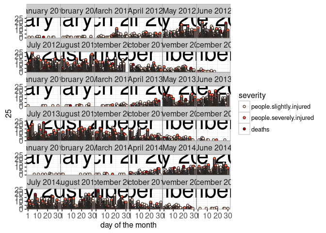
(counter.locations <- data.table(montreal.bikes$counter.locations)[, let(
  lon = coord_X,
  lat = coord_Y
)][])
## id nom nom_comptage
## <char> <char> <char>
## 1: 1 St-Urbain_1 Saint-Urbain
## 2: 2 Brebeuf_1 Brebeuf
## 3: 4 Maisonneuve_1 Maisonneuve_1
## 4: 5 Maisonneuve_2 Maisonneuve_2
## 5: 6 Rachel/Papineau Rachel/Papineau
## 6: 7 University_1 University
## 7: 8 Cote-Ste-Catherine_1 CSC
## 8: 10 Jacques-Cartier_1 Pont_Jacques-Cartier
## 9: 12 Pierre-Dupuy_1 PierDup
## 10: 14 St-Antoine_1 Saint-Antoine
## 11: 15 Viger_1 Viger
## 12: 17 Maisonneuve_3 Maisonneuve_3
## 13: 19 Piste_Notre-Dame Notre-Dame
## 14: 22 Parc_1 Parc
## 15: 23 Rachel/H\xf4tel-de-Ville Rachel/H\xf4tel de Ville
## 16: 29 Boyer_1 Boyer
## 17: 36 Ren\xe9-L\xe9vesque_2 Ren\xe9-L\xe9vesque
## 18: 37 Totem_Laurier Totem_Laurier
## 19: 3 Berri_1 Berri1
## 20: 38 Parc_2 Parc U-Zelt Test
## 21: 39 St-Laurent Saint-Laurent U-Zelt Test
## id nom nom_comptage
## Etat Type Annee_implante coord_X coord_Y
## <char> <char> <char> <num> <num>
## 1: Existant compteur 2014 -73.58888 45.51955
## 2: Existant compteur 2009 -73.57398 45.52741
## 3: \xc0 r\xe9installer compteur 2008 -73.56159 45.51479
## 4: Existant compteur 2008 -73.57508 45.50054
## 5: Existant compteur 2007 -73.56965 45.53036
## 6: Existant compteur 2013 -73.57512 45.50574
## 7: Existant compteur 2010 -73.60783 45.51496
## 8: Existant compteur 2011 -73.55458 45.52560
## 9: Existant compteur 2010 -73.54455 45.49966
## 10: Existant compteur 2013 -73.55779 45.50625
## 11: Existant compteur 2013 -73.55909 45.50714
## 12: Existant compteur 2013 -73.58523 45.49056
## 13: Existant compteur 2013 -73.54404 45.53140
## 14: Existant compteur 2010 -73.58171 45.51346
## 15: Existant compteur 2013 -73.58025 45.51958
## 16: Existant compteur 2013 -73.60523 45.53840
## 17: Existant compteur 2013 -73.55404 45.51697
## 18: Existant totem 2013 -73.58883 45.52777
## 19: Existant compteur 2008 -73.56284 45.51613
## 20: Existant Projet-pilot 2015 -73.58221 45.51370
## 21: Existant Projet-pilot 2015 -73.60311 45.52782
## Etat Type Annee_implante coord_X coord_Y
## lon lat
## <num> <num>
## 1: -73.58888 45.51955
## 2: -73.57398 45.52741
## 3: -73.56159 45.51479
## 4: -73.57508 45.50054
## 5: -73.56965 45.53036
## 6: -73.57512 45.50574
## 7: -73.60783 45.51496
## 8: -73.55458 45.52560
## 9: -73.54455 45.49966
## 10: -73.55779 45.50625
## 11: -73.55909 45.50714
## 12: -73.58523 45.49056
## 13: -73.54404 45.53140
## 14: -73.58171 45.51346
## 15: -73.58025 45.51958
## 16: -73.60523 45.53840
## 17: -73.55404 45.51697
## 18: -73.58883 45.52777
## 19: -73.56284 45.51613
## 20: -73.58221 45.51370
## 21: -73.60311 45.52782
## lon latloc.name.code <- c(
"Berri1"="Berri",
"Brebeuf"="Brébeuf",
CSC="Côte-Sainte-Catherine",
"Maisonneuve_1"="Maisonneuve 1",
"Maisonneuve_2"="Maisonneuve 2",
"Parc"="du Parc",
PierDup="Pierre-Dupuy",
"Rachel/Papineau"="Rachel",
"Saint-Urbain"="Saint-Urbain",
"Totem_Laurier"="Totem_Laurier")
counter.locations[, location := loc.name.code[nom_comptage] ]
velo.counts <- table(counts.dt$location)
(show.locations <- counter.locations[names(velo.counts), on=list(location)])## id nom nom_comptage Etat Type
## <char> <char> <char> <char> <char>
## 1: 3 Berri_1 Berri1 Existant compteur
## 2: 2 Brebeuf_1 Brebeuf Existant compteur
## 3: 8 Cote-Ste-Catherine_1 CSC Existant compteur
## 4: 4 Maisonneuve_1 Maisonneuve_1 \xc0 r\xe9installer compteur
## 5: 5 Maisonneuve_2 Maisonneuve_2 Existant compteur
## 6: 22 Parc_1 Parc Existant compteur
## 7: 12 Pierre-Dupuy_1 PierDup Existant compteur
## 8: 6 Rachel/Papineau Rachel/Papineau Existant compteur
## 9: 1 St-Urbain_1 Saint-Urbain Existant compteur
## 10: 37 Totem_Laurier Totem_Laurier Existant totem
## Annee_implante coord_X coord_Y lon lat location
## <char> <num> <num> <num> <num> <char>
## 1: 2008 -73.56284 45.51613 -73.56284 45.51613 Berri
## 2: 2009 -73.57398 45.52741 -73.57398 45.52741 Brébeuf
## 3: 2010 -73.60783 45.51496 -73.60783 45.51496 Côte-Sainte-Catherine
## 4: 2008 -73.56159 45.51479 -73.56159 45.51479 Maisonneuve 1
## 5: 2008 -73.57508 45.50054 -73.57508 45.50054 Maisonneuve 2
## 6: 2010 -73.58171 45.51346 -73.58171 45.51346 du Parc
## 7: 2010 -73.54455 45.49966 -73.54455 45.49966 Pierre-Dupuy
## 8: 2007 -73.56965 45.53036 -73.56965 45.53036 Rachel
## 9: 2014 -73.58888 45.51955 -73.58888 45.51955 Saint-Urbain
## 10: 2013 -73.58883 45.52777 -73.58883 45.52777 Totem_LaurierThe counter locations above will be plotted below. Note that we use showSelected=month and clickSelects=location.
map.lim <- show.locations[, list(
  range.lat=range(lat),
  range.lon=range(lon)
)]
diff.vec <- sapply(map.lim, diff)
diff.mat <- c(-1, 1) * matrix(diff.vec, 2, 2, byrow=TRUE)
scale.mat <- as.matrix(map.lim) + diff.mat
location.colors <-
  c("#8DD3C7", "#FFFFB3", "#BEBADA", "#FB8072", "#80B1D3", "#FDB462",
    "#B3DE69", "#FCCDE5", "#D9D9D9", "#BC80BD", "#CCEBC5", "#FFED6F")
names(location.colors) <- show.locations$location
counts.per.month.loc <- counts.per.month[show.locations, on=list(location)]
bike.paths <- data.table(montreal.bikes$path.locations)
some.paths <- bike.paths[
  scale.mat[1, "range.lat"] < lat &
    scale.mat[1, "range.lon"] < lon &
    lat < scale.mat[2, "range.lat"] &
    lon < scale.mat[2, "range.lon"]]
mtl.map <- ggplot()+
  theme_bw()+
  theme(
    panel.margin=grid::unit(0, "lines"),
    axis.line=element_blank(), axis.text=element_blank(),
    axis.ticks=element_blank(), axis.title=element_blank(),
    panel.background = element_blank(),
    panel.border = element_blank())+
  coord_equal(xlim=map.lim$range.lon, ylim=map.lim$range.lat)+
  scale_color_manual(values=location.colors)+
  scale_x_continuous(limits=scale.mat[, "range.lon"])+
  scale_y_continuous(limits=scale.mat[, "range.lat"])+
  geom_path(aes(
    lon, lat,
    tooltip=TYPE_VOIE,
    group=paste(feature.i, path.i)),
    color="grey",
    data=some.paths)+
  guides(color="none")+
  geom_text(aes(
    lon, lat,
    label=location),
    clickSelects="location",
    data=show.locations)
mtl.map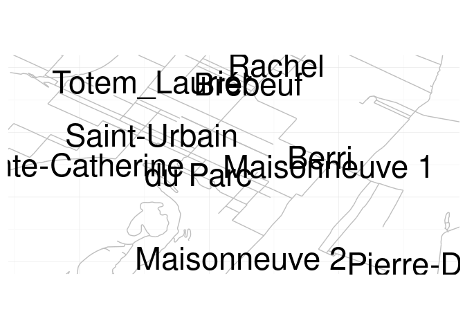
The plot below shows the time period that each counter was in operation. Note that we use geom_tallrect with clickSelects to select the month.
location.ranges <- counts.per.month[0 < count, list(
  min=min(month.POSIXct),
  max=max(month.POSIXct)
), by=location]
accidents.range <- accidents.dt[, data.table(
  location="accidents",
  min=min(date.POSIXct),
  max=max(date.POSIXct))]
MonthSummary <- ggplot()+
  theme_bw()+
  theme_animint(width=450, height=250)+
  xlab("range of dates in data")+
  ylab("data type")+
  scale_color_manual(values=location.colors)+
  guides(color="none")+
  geom_segment(aes(
    min, location,
    xend=max, yend=location,
    color=location),
    clickSelects="location",
    data=location.ranges, alpha=3/4, size=10)+
  geom_segment(aes(
    min, location,
    xend=max, yend=location),
    color=severity.colors[["deaths"]],
    data=accidents.range,
    size=10)
print(MonthSummary)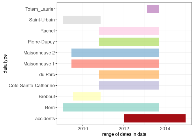
The plot below shows the bike counts at each location and day.
(dates <- counts.dt[, list(
  min.date = date-one.day/2,
  max.date = date+one.day/2,
  locations=sum(!is.na(count))
), by=list(date)][0 < locations])
## date min.date max.date locations
## <POSc> <POSc> <POSc> <int>
## 1: 2009-01-01 06:00:00 2008-12-31 18:00:00 2009-01-01 18:00:00 9
## 2: 2009-01-02 06:00:00 2009-01-01 18:00:00 2009-01-02 18:00:00 9
## 3: 2009-01-03 06:00:00 2009-01-02 18:00:00 2009-01-03 18:00:00 9
## 4: 2009-01-04 06:00:00 2009-01-03 18:00:00 2009-01-04 18:00:00 9
## 5: 2009-01-05 06:00:00 2009-01-04 18:00:00 2009-01-05 18:00:00 9
## ---
## 1604: 2013-09-14 06:00:00 2013-09-13 18:00:00 2013-09-14 18:00:00 8
## 1605: 2013-09-15 06:00:00 2013-09-14 18:00:00 2013-09-15 18:00:00 8
## 1606: 2013-09-16 06:00:00 2013-09-15 18:00:00 2013-09-16 18:00:00 8
## 1607: 2013-09-17 06:00:00 2013-09-16 18:00:00 2013-09-17 18:00:00 8
## 1608: 2013-09-18 06:00:00 2013-09-17 18:00:00 2013-09-18 18:00:00 8(location.labels <- counts.dt[
, .SD[which.max(count)]
, by=list(location)])## location date count month.str
## <fctr> <POSc> <int> <char>
## 1: Berri 2010-06-15 06:00:00 7495 2010-06
## 2: Brébeuf 2010-06-04 06:00:00 9235 2010-06
## 3: Côte-Sainte-Catherine 2013-09-18 06:00:00 3330 2013-09
## 4: Maisonneuve 1 2011-06-17 06:00:00 5355 2011-06
## 5: Maisonneuve 2 2011-06-07 06:00:00 8332 2011-06
## 6: du Parc 2011-09-27 06:00:00 4577 2011-09
## 7: Pierre-Dupuy 2013-07-21 06:00:00 4841 2013-07
## 8: Rachel 2013-05-31 06:00:00 8555 2013-05
## 9: Saint-Urbain 2010-04-27 06:00:00 3856 2010-04
## 10: Totem_Laurier 2013-08-21 06:00:00 4293 2013-08
## loc.lines month.POSIXct month.text day.of.the.month
## <char> <POSc> <char> <int>
## 1: Berri 2010-06-15 June 2010 15
## 2: Brébeuf 2010-06-15 June 2010 4
## 3: Côte\nSainte\nCatherine 2013-09-15 September 2013 18
## 4: Maisonneuve\n1 2011-06-15 June 2011 17
## 5: Maisonneuve\n2 2011-06-15 June 2011 7
## 6: du\nParc 2011-09-15 September 2011 27
## 7: Pierre\nDupuy 2013-07-15 July 2013 21
## 8: Rachel 2013-05-15 May 2013 31
## 9: Saint\nUrbain 2010-04-15 April 2010 27
## 10: Totem\nLaurier 2013-08-15 August 2013 21
## month
## <fctr>
## 1: June 2010
## 2: June 2010
## 3: September 2013
## 4: June 2011
## 5: June 2011
## 6: September 2011
## 7: July 2013
## 8: May 2013
## 9: April 2010
## 10: August 2013TimeSeries <- ggplot()+
theme_bw()+
geom_tallrect(aes(
xmin=date-one.day/2, xmax=date+one.day/2,
clickSelects=date),
data=dates, alpha=1/2)+
geom_line(aes(
date, count, group=location,
showSelected=location,
clickSelects=location),
data=counts.dt)+
scale_color_manual(values=location.colors)+
geom_point(aes(
date, count, color=location,
showSelected=location,
clickSelects=location),
data=counts.dt)+
geom_text(aes(
date, count+200, color=location, label=location,
showSelected=location,
clickSelects=location),
data=location.labels)
print(TimeSeries)## Warning: Removed 407 rows containing missing values (geom_point).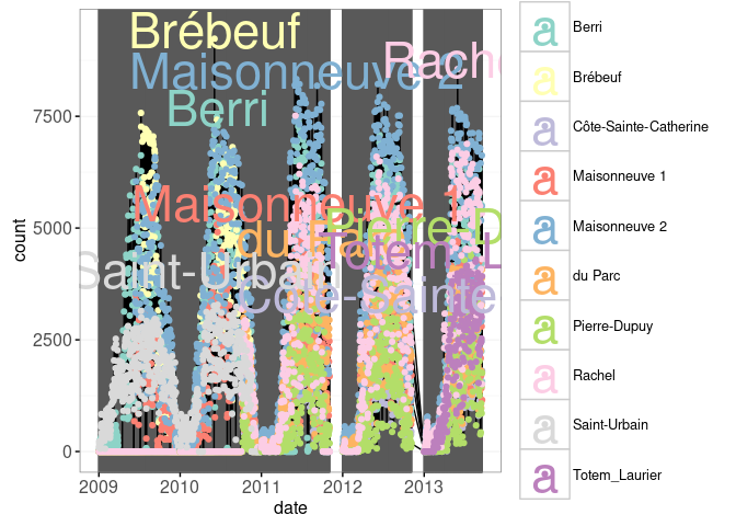
The plot below shows the same data but for each month.
MonthSeries <- ggplot()+
  guides(color="none", fill="none")+
  theme_bw()+
  geom_tallrect(aes(
    xmin=month01.POSIXct, xmax=next01.POSIXct),
    clickSelects="month",
    data=months,
    alpha=1/2)+
  geom_line(aes(
    month.POSIXct, count, group=location,
    color=location),
    showSelected="location",
    clickSelects="location",
    data=counts.per.month)+
  scale_color_manual(values=location.colors)+
  scale_fill_manual(values=location.colors)+
  xlab("month")+
  ylab("bike counts per month")+
  geom_point(aes(
    month.POSIXct, count, fill=location,
    tooltip=paste(
      count, "bikers counted at",
      location, "in", month)),
    showSelected="location",
    clickSelects="location",
    size=5,
    color="black",
    data=counts.per.month)+
  geom_text(aes(
    month.POSIXct, count+5000, color=location, label=location),
    showSelected="location",
    clickSelects="location",
    data=month.labels)
print(MonthSeries)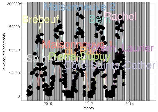
counter.title <- "mean cyclists per day"
accidents.title <- "city-wide accidents"
MonthFacet <- ggplot()+
  ggtitle("All data, select month")+
  guides(color="none", fill="none")+
  theme_bw()+
  facet_grid(facet ~ ., scales="free")+
  theme(panel.margin=grid::unit(0, "lines"))+
  geom_tallrect(aes(
    xmin=month01.POSIXct, xmax=next01.POSIXct),
    clickSelects="month",
    data=data.table(
      city.wide.cyclists,
      facet=counter.title),
    alpha=1/2)+
  geom_line(aes(
    month.POSIXct, mean.per.day, group=location,
    color=location),
    showSelected="location",
    clickSelects="location",
    data=data.table(counts.per.month, facet=counter.title))+
  scale_color_manual(values=location.colors)+
  xlab("month")+
  ylab("")+
  geom_point(aes(
    month.POSIXct, mean.per.day, color=location,
    tooltip=paste(
      count, "cyclists counted at",
      location, "in",
      days, "days of", month,
      sprintf("(mean %d cyclists/day)", as.integer(mean.per.day)))),
    showSelected="location",
    clickSelects="location",
    size=5,
    fill="grey",
    data=data.table(counts.per.month, facet=counter.title))+
  geom_text(aes(
    month.POSIXct, mean.per.day+300, color=location, label=location),
    showSelected="location",
    clickSelects="location",
    data=data.table(month.labels, facet=counter.title))+
  scale_fill_manual(values=severity.colors, breaks=names(severity.colors))+
  geom_bar(aes(
    month.POSIXct, people,
    fill=severity),
    showSelected="severity",
    stat="identity",
    position="identity",
    color=NA,
    data=data.table(accidents.tall, facet=accidents.title))+
  geom_tallrect(aes(
    xmin=month01.POSIXct, xmax=next01.POSIXct,
    tooltip=paste(
      ifelse(deaths==0, "",
      ifelse(deaths==1,
             "1 death,",
             paste(deaths, "deaths,"))),
      ifelse(people.severely.injured==0, "",
      ifelse(people.severely.injured==1,
             "1 person severely injured,",
             paste(people.severely.injured,
                   "people severely injured,"))),
      people.slightly.injured,
      "people slightly injured in",
      month)),
    clickSelects="month",
    alpha=0.5,
    data=data.table(accidents.per.month,
                    facet=accidents.title))
MonthFacet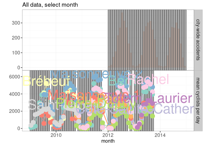
(days.dt <- data.table(
  day.POSIXct=with(months, seq(
    min(month01.POSIXct),
    max(next01.POSIXct),
    by="day"))
)[
, day.of.the.week := strftime(day.POSIXct, "%a")
][])
## day.POSIXct day.of.the.week
## <POSc> <char>
## 1: 2009-01-01 Thu
## 2: 2009-01-02 Fri
## 3: 2009-01-03 Sat
## 4: 2009-01-04 Sun
## 5: 2009-01-05 Mon
## ---
## 2188: 2014-12-28 Sun
## 2189: 2014-12-29 Mon
## 2190: 2014-12-30 Tue
## 2191: 2014-12-31 Wed
## 2192: 2015-01-01 Thu## The following only works in locales with English days of the week.
(weekend.dt <- days.dt[
day.of.the.week %in% c("Sat", "Sun")
][, let(
month.text = strftime(day.POSIXct, "%B %Y"),
day.of.the.month = as.integer(strftime(day.POSIXct, "%d"))
)][
, month := factor(month.text, month.levs)
][])## day.POSIXct day.of.the.week month.text day.of.the.month month
## <POSc> <char> <char> <int> <fctr>
## 1: 2009-01-03 Sat January 2009 3 January 2009
## 2: 2009-01-04 Sun January 2009 4 January 2009
## 3: 2009-01-10 Sat January 2009 10 January 2009
## 4: 2009-01-11 Sun January 2009 11 January 2009
## 5: 2009-01-17 Sat January 2009 17 January 2009
## ---
## 622: 2014-12-14 Sun December 2014 14 December 2014
## 623: 2014-12-20 Sat December 2014 20 December 2014
## 624: 2014-12-21 Sun December 2014 21 December 2014
## 625: 2014-12-27 Sat December 2014 27 December 2014
## 626: 2014-12-28 Sun December 2014 28 December 2014counter.title <- "cyclists per day"
DaysFacet <- ggplot()+
ggtitle("Selected month (weekends in grey)")+
geom_tallrect(aes(
xmin=day.of.the.month-0.5, xmax=day.of.the.month+0.5,
key=paste(day.POSIXct)),
showSelected="month",
fill="grey",
color="white",
data=weekend.dt)+
guides(color="none")+
theme_bw()+
facet_grid(facet ~ ., scales="free")+
geom_line(aes(
day.of.the.month, count, group=location,
key=location,
color=location),
showSelected=c("location", "month"),
clickSelects="location",
chunk_vars=c("month"),
data=data.table(counts.dt, facet=counter.title))+
scale_color_manual(values=location.colors)+
ylab("")+
geom_point(aes(
day.of.the.month, count, color=location,
key=paste(day.of.the.month, location),
tooltip=paste(
count, "cyclists counted at",
location, "on",
date)),
showSelected=c("location", "month"),
clickSelects="location",
size=5,
chunk_vars=c("month"),
fill="white",
data=data.table(counts.dt, facet=counter.title))+
scale_fill_manual(values=severity.colors, breaks=names(severity.colors))+
geom_text(aes(
15, 23, label=month, key=1),
showSelected="month",
data=data.table(months, facet=accidents.title))+
scale_x_continuous("day of the month", breaks=c(1, 10, 20, 30))+
geom_text(aes(
day.of.the.month, count+500, color=location, label=location,
key=location),
showSelected=c("location", "month"),
clickSelects="location",
data=data.table(day.labels, facet=counter.title))+
geom_point(aes(
day.of.the.month, accident.i,
key=paste(date.str, accident.i),
tooltip=paste(
ifelse(deaths==0, "",
ifelse(deaths==1,
"1 death,",
paste(deaths, "deaths,"))),
ifelse(people.severely.injured==0, "",
ifelse(people.severely.injured==1,
"1 person severely injured,",
paste(people.severely.injured,
"people severely injured,"))),
people.slightly.injured,
"people slightly injured at",
ifelse(is.na(street.number), "", street.number),
street, "/", cross.street,
date.str, time.str),
fill=severity),
showSelected="month",
size=4,
chunk_vars=c("month"),
data=data.table(accidents.cumsum, facet=accidents.title))
DaysFacet## Warning: Removed 407 rows containing missing values (geom_point).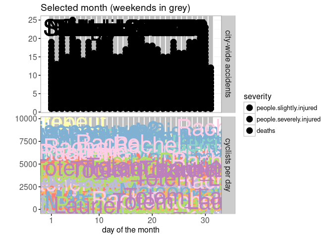
animint(
  MonthFacet,
  DaysFacet,
  MonthSummary,
  selector.types=list(severity="multiple"),
  duration=list(month=2000),
  first=list(
    location="Berri",
    month="September 2012"),
  time=list(variable="month", ms=5000))#buggy.
Chapter summary and exercises
Exercises:
- Change location to a multiple selection variable.
- Add a plot for the map to the data viz.
- On the map, draw a circle for each location, with size that changes based on the
countof the accidents in the currently selectedmonth. - On the
MonthSummaryplot, add a background rectangle that can be used to select themonth. - Remove the
MonthSummaryplot and add a similar visualization as a third panel in theMonthFacetplot.
Next, Chapter 10 explains how to visualize the K-Nearest-Neighbors machine learning model.
