Chapter 16, Change-point detection
In this chapter we will explore several data visualizations of supervised changepoint detection models.
Chapter outline:
- We begin by making several static visualizations of the
intregdata set. - We then create an interactive visualization in which one plot can be click to select the number of changepoints/segments, and the other plot shows the corresponding model.
- We end by showing a static visualization of the max margin linear regression model, and suggesting exercises about creating an interactive version.
Static figures
We begin by loading the intreg data set.
library(animint2)
data(intreg)
str(intreg)
## List of 7
## $ model :'data.frame': 6 obs. of 5 variables:
## ..$ line : Factor w/ 3 levels "regression","limit",..: 1 2 2 3 3 3
## ..$ min.L : num [1:6] -1.4001 -0.1494 -2.6508 -1.365 0.0418 ...
## ..$ max.L : num [1:6] 2.139 3.39 0.888 -0.114 1.293 ...
## ..$ min.feature: num [1:6] -2.48 -2.48 -2.48 -2.15 -1.8 ...
## ..$ max.feature: num [1:6] -1.58 -1.58 -1.58 -2.15 -1.8 ...
## $ annotations:'data.frame': 8 obs. of 5 variables:
## ..$ signal : Factor w/ 7 levels "10.9","11.2",..: 2 5 5 6 7 4 3 1
## ..$ first.base: int [1:8] 55103411 140080934 9346283 38525107 80139652 40489367 34972003 20997136
## ..$ last.base : int [1:8] 161558770 201712984 80316522 95564984 180580302 109068985 103694899 107898044
## ..$ annotation: Factor w/ 2 levels "0breakpoints",..: 1 2 2 2 1 2 1 1
## ..$ logratio : num [1:8] 0.985 0.985 0.985 0.985 0.985 ...
## $ intervals :'data.frame': 7 obs. of 4 variables:
## ..$ signal : Factor w/ 7 levels "10.9","11.2",..: 5 2 6 7 4 3 1
## ..$ feature: num [1:7] -2.15 -1.8 -2.07 -2.48 -1.92 ...
## ..$ min.L : num [1:7] -1.365 0.0418 -2.4514 -3.2211 -1.7404 ...
## ..$ max.L : num [1:7] 1.14 Inf 2.27 Inf 2.28 ...
## $ selection :'data.frame': 98 obs. of 5 variables:
## ..$ signal : Factor w/ 7 levels "4.2","11.2","4.3",..: 1 1 1 1 1 1 1 1 1 1 ...
## ..$ min.L : num [1:98] -Inf -3.57 -3.3 -3.26 -3 ...
## ..$ max.L : num [1:98] -3.57 -3.3 -3.26 -3 -2.88 ...
## ..$ segments: int [1:98] 20 19 16 15 14 13 11 9 8 7 ...
## ..$ cost : num [1:98] 2 2 2 2 1 1 1 1 1 1 ...
## $ segments :'data.frame': 1470 obs. of 5 variables:
## ..$ signal : Factor w/ 7 levels "4.2","11.2","4.3",..: 1 1 1 1 1 1 1 1 1 1 ...
## ..$ segments : int [1:1470] 1 2 2 3 3 3 4 4 4 4 ...
## ..$ first.base: num [1:1470] 1.47e+06 1.47e+06 4.52e+07 1.47e+06 1.14e+08 ...
## ..$ last.base : num [1:1470] 2.43e+08 4.52e+07 2.43e+08 1.14e+08 1.63e+08 ...
## ..$ mean : num [1:1470] -0.0209 0.3512 -0.1 0.1312 -0.4535 ...
## $ breaks :'data.frame': 1330 obs. of 3 variables:
## ..$ signal : Factor w/ 7 levels "4.2","11.2","4.3",..: 1 1 1 1 1 1 1 1 1 1 ...
## ..$ base : num [1:1330] 4.52e+07 1.14e+08 1.63e+08 4.52e+07 1.14e+08 ...
## ..$ segments: int [1:1330] 2 3 3 4 4 4 5 5 5 5 ...
## $ signals :'data.frame': 1314 obs. of 3 variables:
## ..$ signal : Factor w/ 7 levels "4.2","11.2","4.3",..: 1 1 1 1 1 1 1 1 1 1 ...
## ..$ base : int [1:1314] 1472476 2063049 3098882 7177474 8179390 8916469 9470069 11607188 11885382 12173642 ...
## ..$ logratio: num [1:1314] 0.44 0.459 0.341 0.336 0.317 ...As shown above, it is a named list of 7 related data.frames. We begin our exploration of these data by plotting the signals in separate facets.
data.color <- "grey50"
gg.signals <- ggplot()+
  theme_bw()+
  facet_grid(signal ~ ., scales="free")+
  geom_point(aes(
    base/1e6, logratio,
    showSelected="signal"),
    color=data.color,
    data=intreg$signals)
print(gg.signals)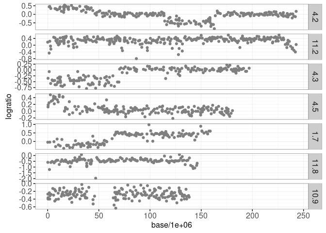
Each data point plotted above shows an approximate measurement of DNA copy number (logratio), as a function of base position on a chromosome. Such data come from high-throughput assays which are important for diagnosing certain types of cancer such as neuroblastoma.
An important part of the diagnosis is detecting “breakpoints” or abrupt changes, within a given chromosome (panel). It is clear from the plot above that there are several breakpoint in these data. In particular signal 4.2 appears to have three breakpoints, signal 4.3 appears to have one, etc. In fact these data come from medical doctors at the Institute Curie (Paris, France) who have visually annotated regions with and without breakpoints. These data are available as intreg$annotations and are plotted below.
breakpoint.colors <- c("1breakpoint"="#ff7d7d", "0breakpoints"='#f6f4bf')
gg.ann <- gg.signals+
  scale_fill_manual(values=breakpoint.colors)+
  geom_tallrect(aes(
    xmin=first.base/1e6, xmax=last.base/1e6,
    fill=annotation),
    color="grey",
    alpha=0.5,
    data=intreg$annotations)
print(gg.ann)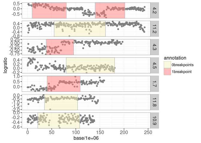
The plot above shows yellow regions where the doctors have determined that there are no significant breakpoints, and red regions where there is one breakpoint. The goal in analyzing these data is to learn from the limited labeled data (colored regions) and provide consistent breakpoint predictions throughout (even in un-labeled regions).
In order to detect these breakpoints we have fit some maximum likelihood segmentation models, using the efficient algorithm implemented in jointseg::Fpsn. The segment means are available in intreg$segments and the predicted breakpoints are available in intreg$breaks. For each signal there is a sequence of models from 1 to 20 segments. First let’s zoom in on one signal:
sig.name <- "4.2"
show.segs <- 7
sig.labels <- subset(intreg$annotations, signal==sig.name)
gg.one <- ggplot()+
  theme_bw()+
  theme(panel.margin=grid::unit(0, "lines"))+
  geom_tallrect(aes(
    xmin=first.base/1e6, xmax=last.base/1e6,
    fill=annotation),
    color="grey",
    alpha=0.5,
    data=sig.labels)+
  geom_point(aes(
    base/1e6, logratio),
    color=data.color,
    data=subset(intreg$signals, signal==sig.name))+
  scale_fill_manual(values=breakpoint.colors)
print(gg.one)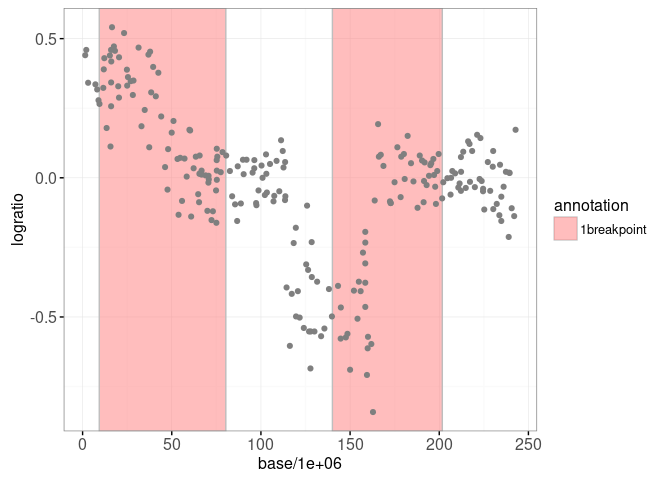
We plot some of these models for one of the signals below:
library(data.table)
sig.segs <- data.table(
  intreg$segments)[signal == sig.name & segments <= show.segs]
sig.breaks <- data.table(
  intreg$breaks)[signal == sig.name & segments <= show.segs]
model.color <- "green"
gg.models <- gg.one+
  facet_grid(segments ~ .)+
  geom_segment(aes(
    first.base/1e6, mean,
    xend=last.base/1e6, yend=mean),
    color=model.color,
    data=sig.segs)+
  geom_vline(aes(
    xintercept=base/1e6),
    color=model.color,
    linetype="dashed",
    data=sig.breaks)
print(gg.models)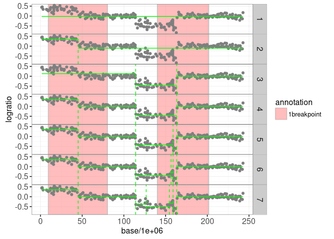
The plot above shows the maximum likelihood segmentation models in green (from one to six segments). Below we use the penaltyLearning::labelError function to compute the label error, which quantifies which models agree with which labels.
sig.models <- data.table(segments=1:show.segs, signal=sig.name)
sig.errors <- penaltyLearning::labelError(
  sig.models, sig.labels, sig.breaks,
  change.var="base",
  label.vars=c("first.base", "last.base"),
  model.vars="segments",
  problem.vars="signal")
The sig.errors$label.errors data.table contains one row for every (model,label) combination. The status column can be used to show the label error: false negative for too few changes, false positive for too many changes, or correct for the right number of changes.
gg.models+
  geom_tallrect(aes(
    xmin=first.base/1e6, xmax=last.base/1e6,
    linetype=status),
    data=sig.errors$label.errors,
    color="black",
    size=1,
    fill=NA)+
  scale_linetype_manual(
    "error type",
    values=c(
      correct=0,
      "false negative"=3,
      "false positive"=1))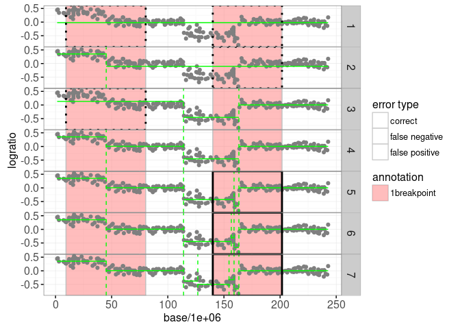
Looking at the label error plot above, it is clear that the model with four segments should be selected, because it achieves zero label errors. There are a number of criteria that can be used to select which one of these models is best. One way to do that is by selecting the model with s segments is S*(λ)=Ls + λ * s, where Ls is the total loss of the model with s segments, and λ is a non-negative penalty. In the plot below we show the model selection function S*(λ) for this data set:
sig.selection <- data.table(
  intreg$selection)[signal == sig.name & segments <= show.segs]
gg.selection <- ggplot()+
  theme_bw()+
  geom_segment(aes(
    min.L, segments,
    xend=max.L, yend=segments),
    data=sig.selection)+
  xlab("log(lambda)")
print(gg.selection)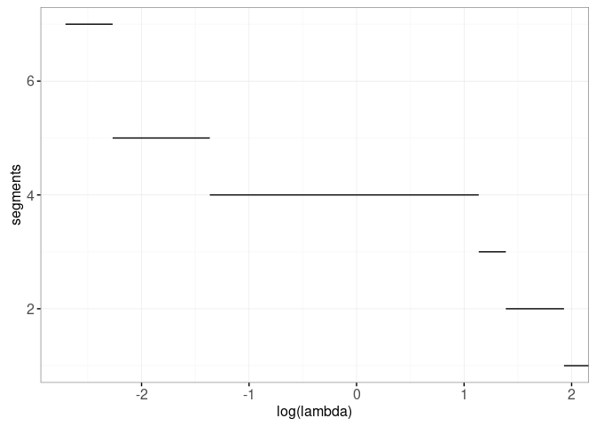
It is clear from the plot above that the model selection function is decreasing. In the next section we make an interactive version of these two plots where we can actually click on the model selection plot in order to select the model.
Interactive figures for one signal
We will create an interactive figure for one signal by adding a geom_tallrect with clickSelects=segments to the plot above:
interactive.selection <- gg.selection+
  geom_tallrect(aes(
    xmin=min.L, xmax=max.L),
    clickSelects="segments",
    data=sig.selection,
    color=NA,
    fill="black",
    alpha=0.5)
print(interactive.selection)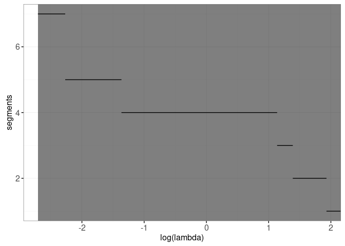
We will combine that with the non-facetted version of the data/models plot below, in which we have added showSelected=segments to the model geoms:
interactive.models <- gg.one+
  geom_segment(aes(
    first.base/1e6, mean,
    xend=last.base/1e6, yend=mean),
    showSelected="segments",
    color=model.color,
    data=sig.segs)+
  geom_vline(aes(
    xintercept=base/1e6),
    showSelected="segments",
    color=model.color,
    linetype="dashed",
    data=sig.breaks)+
  geom_tallrect(aes(
    xmin=first.base/1e6, xmax=last.base/1e6,
    linetype=status),
    showSelected="segments",
    data=sig.errors$label.errors,
    size=2,
    color="black",
    fill=NA)+
  scale_linetype_manual(
    "error type",
    values=c(
      correct=0,
      "false negative"=3,
      "false positive"=1))
print(interactive.models)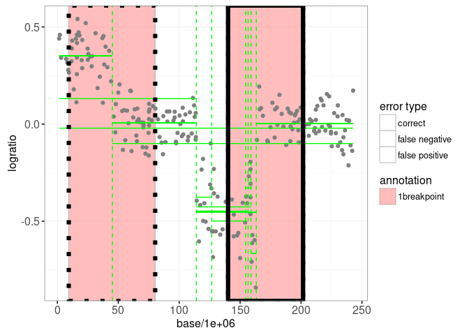
Of course the plot above is not very informative because it is not interactive. Below we combine the two interactive ggplots in a single linked animint:
animint(
  models=interactive.models+
    ggtitle("Selected model"),
  selection=interactive.selection+
    ggtitle("Click to select number of segments"))
Note that in the data viz above the model with 6 segments is not selectable for any value of lambda, so there is no way to click on the plot to select that model. However it is possible to select the model using the segments selection menu (click “Show selection menus” at the bottom of the data viz).
Static max margin regression plot
Another part of this data set is intreg$intervals which has one row for every signal. The columns min.L and max.L indicate the min/max values of the target interval, which is the largest range of log(penalty) values with minimum label errors. Below we plot this interval as a function of a feature of the data (log number of data points):
gg.intervals <- ggplot()+
  geom_segment(aes(
    feature, min.L,
    xend=feature, yend=max.L),
    size=2,
    data=intreg$intervals)+
  geom_text(aes(
    feature, min.L, label=signal,
    color=ifelse(signal==sig.name, "black", "grey50")),
    vjust=1,
    data=intreg$intervals)+
  scale_color_identity()+
  ylab("output log(lambda)")+
  xlab("input feature x")
print(gg.intervals)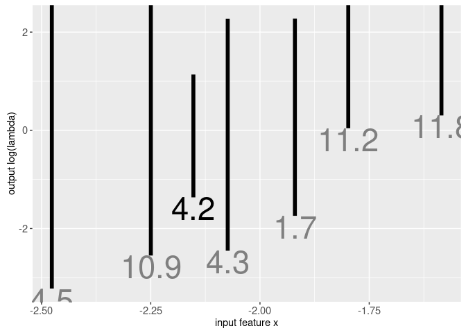
The target intervals in the plot above denote the region of log(lambda) space that will select a model with minimum label errors. There is one interval for each signal; we made an animint in the previous section for the signal indicated in black text. Machine learning algorithms can be used to find a penalty function that intersects each of the intervals, and maximizes the margin (the distance between the regression function and the nearest interval limit). Data for the linear max margin regression function are in intreg$model which is shown in the plot below:
gg.mm <- gg.intervals+
  geom_segment(aes(
    min.feature, min.L,
    xend=max.feature, yend=max.L,
    linetype=line),
    color="red",
    size=1,
    data=intreg$model)+
  scale_linetype_manual(
    values=c(
      regression="solid",
      margin="dotted",
      limit="dashed"))
print(gg.mm) 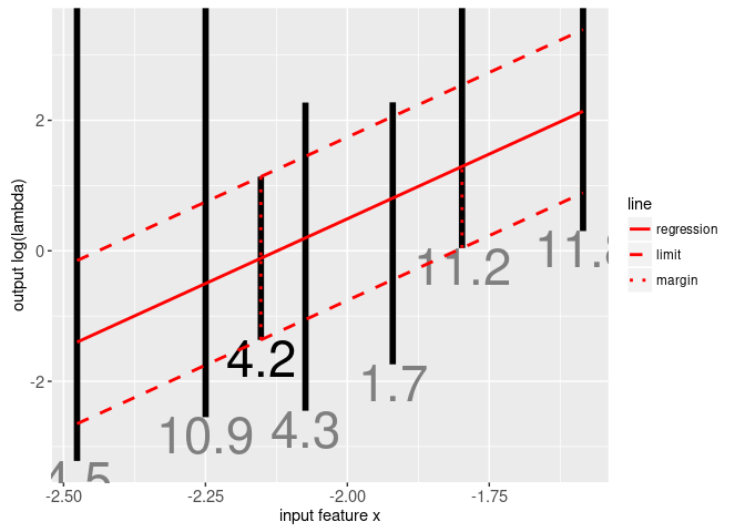
The plot above shows the linear max margin regression function f(x) as the solid red line. It is clear that it intersects each of the black target intervals, and maximizes the margin (red vertical dotted lines). For more information on the subject of supervised changepoint detection, please see my useR 2017 tutorial.
Now that you know how to visualize each of the seven parts of the intreg data set, the rest of the chapter is devoted to exercises.
Chapter summary and exercises
Exercises:
- Add a
geom_textwhich shows the currently selected signal name at the top of the plot, ininteractive.modelsin the first animint above. - Make an animint with two plots that shows the data set that corresponds to each interval on the max margin regression plot. One plot should show an interactive version of the max margin regression plot where you can click on an interval to select a signal. The other plot should show the data set for the currently selected signal.
- In the animint you created in the previous exercise, add a third plot with the model selection function for the currently selected signal.
- Re-design the previous animint so that instead of using a third plot, add a facet to the max margin regression regression plot such that the log(lambda) axes are aligned. Add another facet that shows the number of incorrect labels (
intreg$selection$cost) for each log(lambda) value. - Add geoms for selecting the number of segments. Clicking the model selection plot should select the number of segments, which should update the displayed model and label errors on the plot of the data for the currently selected signal. Furthermore add a visual indication of the selected model to the max margin regression plot. The result should look something like this.
- Make another data viz by starting with the facetted
gg.signalsplot in the beginning of this chapter. Add a plot that can be used to select the number of segments for each signal. For each signal in the facetted plot of the data, show the currently selected model for that signal (there should be a separate selection variable for each signal – you can use named clickSelects/showSelected as explained in Chapter 14). The result should look something like this.
Next, Chapter 17 explains how to visualize the K-means clustering algorithm.
